Part III · The Deep Theory
Hamilton Cycles
A Hamilton cycle is a round trip that visits every vertex exactly once. After this chapter you will know why no clean test for one is expected to exist, and you will own the classic toolbox that guarantees one anyway: Dirac's degree bound, Chvátal's complete answer for degree sequences, and Fleischner's theorem on squared graphs.
The other grand tour
Picture a road network: towns as vertices, roads as edges. Two natural "grand tour" questions come up. Can you take a round trip that drives along every road exactly once? And can you take a round trip that visits every town exactly once? The two questions sound like twins. They are not.
The first question, about edges, was settled back in Chapter 1. A closed walk that uses every edge exactly once is an Euler tour, and a connected graph has one exactly when every vertex has even degree[4]. That is a complete answer. You can check it by glancing at each vertex and counting.
The second question, about vertices, is this chapter's subject, and it has no such answer. Nobody knows a clean test, and there are strong reasons to believe none exists.
A Hamilton cycle of a graph \(G\) is a cycle in \(G\) that contains every vertex of \(G\): a round trip visiting each vertex exactly once and returning to its start. A graph that has a Hamilton cycle is called hamiltonian. A Hamilton path is the one-way version: a path containing every vertex, with no obligation to return home. In plain terms: an Euler tour uses every edge once; a Hamilton cycle visits every vertex once.
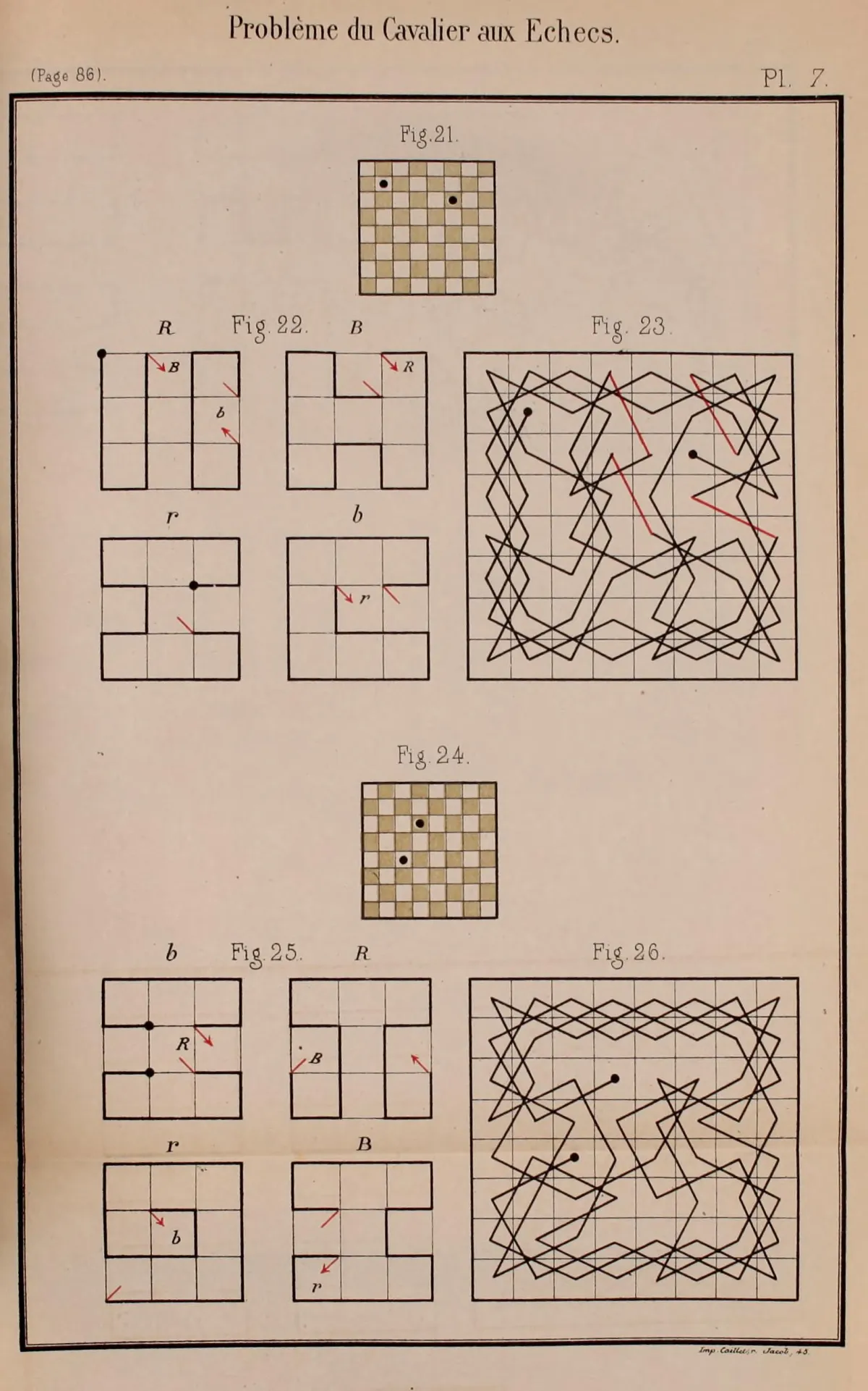
The name honours W. R. Hamilton, who in 1857 sold a puzzle game asking players to find exactly such tours on the graph of the dodecahedron, the twelve-sided die shape[5]. Figure 10.1 shows the graph and one winning tour. The same family of puzzles is much older than graph theory: asking whether a knight can visit every square of a chessboard exactly once and hop back to its start is a Hamilton cycle question in disguise. So is the puzzle of listing all the on/off settings of a row of switches so that each step flips just one switch: that is a Hamilton cycle in the cube-like graph whose vertices are the settings.
Why is the vertex tour so much harder than the edge tour? An Euler tour has a local certificate: the even-degree condition can be checked one vertex at a time, and any failure points at its own culprit. A Hamilton cycle has no known local certificate. Whether a tour can thread through your corner of the graph depends on choices made far away. Deciding whether a graph is hamiltonian is NP-hard: it was among the first problems recognized as computationally intractable in this sense, and no efficient method for it is expected to exist[5]. One word, edge versus vertex, separates trivial from intractable.
Genome assembly ran head-first into this divide. DNA sequencers read a genome as billions of short overlapping fragments, and software must stitch them back together. The naive model makes each fragment a vertex and asks for a path visiting every vertex once: a Hamilton path problem, hopeless at that scale. The fix that modern assemblers use is to rebuild the graph so that fragments become edges, turning the task into an Euler path problem, which is solvable fast. Compeau, Pevzner and Tesler describe this de Bruijn graph reformulation as what turned genome assembly into a tractable computation[6]. Working scientists deliberately migrated their problem from the hard side of this chapter's divide to the easy side of Chapter 1's. The same divide shows up in street routing: the mail carrier's "cover every street" problem is solved exactly by Euler tours plus matching theory[7], while the salesman's "visit every customer" problem sits on the hard side.
So what does a chapter about an intractable problem do? It maps the border. Instead of one perfect characterization, we build a toolbox of sufficient conditions: checkable properties that guarantee a Hamilton cycle exists, even though many hamiltonian graphs satisfy none of them. The plan follows Diestel's Chapter 10: the classic sufficient conditions (Dirac, Chvátal–Erdős, Asratian–Khachatrian, Tutte)[1], then Chvátal's complete answer to "when do the degrees alone force a tour?"[2], and finally Fleischner's theorem on squares of graphs[3]. Almost every theorem comes paired with an example showing it cannot be improved. That back-and-forth between theorem and counterexample is the real lesson.
Modern genome assemblers rebuild the fragment graph so that fragments become edges instead of vertices. Why is that the winning move?
New notation in this chapter
| Symbol | Read it as | Meaning | Tiny example |
|---|---|---|---|
| \(G^d\) | "the d-th power of G" | Same vertices as \(G\); an edge joins two vertices whenever they are at distance at most \(d\) in \(G\) (reachable in at most \(d\) steps). | If \(G\) is the path \(a\,b\,c\,d\), then \(G^2\) adds \(ac\) and \(bd\), but not \(ad\) (distance 3). |
| \(G^2\) | "the square of G" | The case \(d=2\): keep all edges of \(G\), add an edge between every pair of vertices exactly two steps apart. | The square of the path \(v_1 v_2 v_3 v_4 v_5\) adds \(v_1v_3\), \(v_2v_4\), \(v_3v_5\). |
| \((d_1, \dots, d_n)\) | "the degree sequence" | All \(n\) vertex degrees of a graph, sorted in increasing order: \(d_1 \le d_2 \le \dots \le d_n\). | Two triangles sharing a vertex (the bowtie): \((2,2,2,2,4)\). |
| \(v^+\) | "the successor of v" | Fix a direction of travel around a cycle; \(v^+\) is the vertex that comes right after \(v\). | On the cycle \(v_1 v_2 v_3 v_1\), travelling in index order, \(v_1^+ = v_2\). |
| \(V^+\) | "V plus" | The set of successors of all vertices in a set \(V\): \(V^+ = \{v^+ : v \in V\}\). | On that same triangle, \(\{v_1, v_2\}^+ = \{v_2, v_3\}\). |
| \(t\)-tough | "t tough" | Deleting any separating set \(S\) of vertices leaves at most \(|S|/t\) connected pieces. Larger \(t\) means harder to shatter. | A cycle is 1-tough: deleting \(k\) vertices leaves at most \(k\) arcs. |
| \(G * K^1\) | "G joined with K one" | Add one new vertex to \(G\) and connect it to every vertex of \(G\). | A Hamilton path in \(G\) becomes a Hamilton cycle in \(G * K^1\), closed through the new vertex. |
| \(\|X, Y\|\) | "the number of X–Y edges" | The count of edges with one end in \(X\) and the other in \(Y\). | In \(K_{2,3}\) with classes \(X\) and \(Y\): \(\|X,Y\| = 6\). |
Recalled from earlier chapters, one clause each: \(|G|\) is the order of \(G\), its number of vertices; \(d(v)\) is the degree of \(v\), its number of neighbours; \(\delta(G)\) is the minimum degree, the smallest degree in the graph; \(N(v)\) is the neighbourhood of \(v\), the set of vertices joined to \(v\) by an edge; \(\alpha(G)\) is the independence number, the size of the largest set of pairwise non-adjacent vertices; \(\kappa(G)\) is the connectivity, the smallest number of vertex deletions that disconnect the graph; \(G - S\) is the graph left after deleting the vertex set \(S\) and all edges touching it; \(K^n\) is the complete graph on \(n\) vertices (Diestel's notation; many other books write \(K_n\)); and \(K_{2,3}\) is the complete bipartite graph with classes of sizes 2 and 3, all six cross edges present and no edges inside a class.
Travel the cycle \(v_1 v_2 v_3 v_4 v_5 v_1\) in index order. What is \(\{v_2, v_5\}^+\)?
Dirac's theorem: own half the graph
What is the crudest thing that could force a Hamilton cycle? Sheer quantity of edges. If every vertex knows enough of the graph, a tour should have no way to get stuck. The founding theorem of the subject makes "enough" exact.
Every graph \(G\) with \(|G| = n \ge 3\) vertices and minimum degree \(\delta(G) \ge n/2\) has a Hamilton cycle[1]. In words: if every single vertex is adjacent to at least half of all the vertices, a full round trip exists.
The proof idea is short enough to enjoy in full. First, the degree bound forces \(G\) to be connected: any two vertices either touch or have a common neighbour, because their neighbourhoods are each too big (at least \(n/2\) vertices) to avoid each other inside a graph of \(n\) vertices. Now take a longest path \(P = v_0 v_1 \dots v_k\). Every neighbour of the endpoint \(v_0\) must lie on \(P\): if \(v_0\) had a neighbour off the path, we could extend \(P\) and it was not longest. The same holds for the other endpoint \(v_k\).
Now count. Among the \(k \lt n\) edges of the path, at least \(n/2\) have their right end adjacent to \(v_0\), and at least \(n/2\) have their left end adjacent to \(v_k\). Two sets of size \(n/2\) inside fewer than \(n\) slots must overlap: some edge \(v_i v_{i+1}\) of the path is doubly good, meaning \(v_0 v_{i+1}\) and \(v_i v_k\) are both edges of \(G\). Those two chords rewire the path into a cycle through all its vertices: travel \(v_0 \to v_{i+1} \to \dots \to v_k\), jump the chord to \(v_i\), travel backwards \(v_i \to \dots \to v_0\). Figure 10.2 shows the surgery. Finally, this cycle must contain every vertex of \(G\): if some vertex were left out, connectivity would attach it to the cycle, and unrolling the cycle at the attachment point would produce a path longer than \(P\). Contradiction, so the cycle is a Hamilton cycle.
Is the bound \(n/2\) just an artifact of the proof? No. It is exactly right, and the counterexample is worth memorizing. Take two complete graphs, each on \(\lceil n/2 \rceil\) vertices (that is \(n/2\) rounded up), and glue them together at a single shared vertex. Figure 10.3 shows the smallest case, \(n = 5\): two triangles sharing a vertex, the bowtie. Every vertex has degree at least \(\lfloor n/2 \rfloor\), which is \(n/2\) rounded down, so the graph misses Dirac's bound by the smallest possible amount. And it has no Hamilton cycle: any round trip through both halves would have to pass through the shared vertex twice, which a cycle never does. So \(n/2\) cannot be relaxed even to \(\lfloor n/2 \rfloor\). In effect, Dirac's bound is exactly high enough to guarantee the graph is 2-connected (no single vertex whose removal disconnects it), which every hamiltonian graph must be.
Reading Dirac's theorem backwards. It promises a Hamilton cycle when \(\delta(G) \ge n/2\); it says nothing when \(\delta(G) \lt n/2\). The 5-cycle in Figure 10.4 is hamiltonian with minimum degree 2, far below \(5/2\). None of this chapter's conditions is necessary. Only two properties in this chapter are necessary for a Hamilton cycle (being 2-connected, and being 1-tough, defined below), and neither is sufficient. Sufficient conditions promise; they never forbid.
Thinking a big constant minimum degree helps. "Every vertex has at least 1000 neighbours" forces nothing: glue two complete graphs on 1001 vertices at a shared vertex and you get a non-hamiltonian graph of minimum degree 1000. The bound in Dirac's theorem must scale with the graph: it is the fraction \(n/2\), not the raw size of the number, that does the work.
In which graph does Dirac's theorem guarantee a Hamilton cycle?
The bowtie, two triangles glued at a shared vertex, has no Hamilton cycle. What is the reason?
Two more angles: connectivity and local degrees
Degrees are one axis. What else might force a tour? A natural guess is connectivity: the minimum number of vertices you must delete to disconnect the graph, written \(\kappa(G)\) and studied in Chapter 3. A highly connected graph is hard to cut apart, so surely a tour can always find a way through?
No amount of connectivity suffices, and the counterexample family is simple. Consider the complete bipartite graphs \(K_{k,\,k+1}\): a class of \(k\) vertices, a class of \(k+1\) vertices, all cross edges. This graph is \(k\)-connected. But any cycle in it must alternate between the two classes, so it uses the small class at most \(k\) times and has length at most \(2k\): too short to cover all \(2k+1\) vertices. Figure 10.5 shows the smallest case, \(K_{2,3}\), together with the cleanest way to see its failure: deleting the two left vertices strands the three right vertices as three separate pieces. A cycle can never be shattered that badly by two deletions, so no Hamilton cycle was ever there.
Notice what witnessed the failure of \(K_{2,3}\): a large set of mutually non-adjacent vertices, namely \(\{w_1, w_2, w_3\}\). The independence number \(\alpha(G)\), the size of the largest such set (from Chapter 5), measures how spread out a graph is. \(K_{2,3}\) has \(\alpha = 3\) but \(\kappa = 2\): more spread out than it is connected. Chvátal and Erdős discovered that this comparison is exactly the right one.
Every graph \(G\) with \(|G| \ge 3\) and \(\alpha(G) \le \kappa(G)\) has a Hamilton cycle[1]. In words: if the graph is at least as connected as it is spread out, a full round trip exists.
The proof idea introduces a trick used throughout this chapter: travel a longest cycle in a fixed direction and study successors. Take a longest cycle \(C\), and suppose it misses some vertex. That vertex lives in some component \(D\) of \(G - C\), the graph left after removing \(C\)'s vertices. Look at the attachment points: the vertices of \(C\) that have a neighbour in \(D\). Because deleting all of them cuts \(D\) off from the rest, there are at least \(\kappa(G)\) of them. Because \(C\) is longest, no two attachment points can be consecutive on \(C\) (otherwise we could detour through \(D\) between them and lengthen the cycle). Now the punchline: the set of successors of the attachment points, one step further along \(C\), turns out to be an independent set, and it stays independent when you add one vertex of \(D\) to it. That gives an independent set of size at least \(\kappa(G) + 1 \gt \alpha(G)\), which is a contradiction. So \(C\) missed nothing, and it is a Hamilton cycle.
Both hypotheses of Dirac's theorem and the Chvátal–Erdős condition are global: they mention \(n\), or compare two whole-graph parameters. Asratian and Khachatrian found something different in kind: a condition you can check by looking only at small neighbourhoods, never at the whole graph.
A connected graph \(G\) with \(|G| \ge 3\) is hamiltonian if every induced path \(u\,v\,w\) satisfies \(d(u) + d(w) \ \ge\ |N(u) \cup N(v) \cup N(w)|\)[1]. Here an induced path \(u\,v\,w\) means \(v\) is adjacent to both \(u\) and \(w\), but \(u\) and \(w\) are not adjacent to each other. In words: in every such three-vertex stretch, the two outer degrees together must be at least the size of the combined neighbourhood of all three vertices.
A small identity makes the condition readable: \(d(u) + d(w) = |N(u) \cup N(w)| + |N(u) \cap N(w)|\), because vertices in both neighbourhoods get counted twice on the left. Feeding this in, the hypothesis forces the two ends of every induced path \(u\,v\,w\) to have at least two common neighbours: \(v\) is always one, and the condition forces a second. The proof then runs the longest-cycle machinery again: take a longest cycle \(C\), a vertex \(u\) off it with neighbour set \(V\) on \(C\), and the successor set \(V^+\). Longest-cycle arguments make each stretch \(u\,v\,v^+\) an induced path and forbid certain edges and shared neighbours around \(V^+\). Double-counting the edges between \(V\) and \(V^+\), written \(\|V, V^+\|\), then produces the absurd conclusion \(\|V, V^+\| \le \|V, V^+\| - |V|\). The full bookkeeping is in Diestel §10.1[1].
Two things make this theorem more than a curiosity. It strictly strengthens Dirac's theorem: whenever \(\delta(G) \ge n/2\), the local condition holds automatically. And unlike any condition that mentions \(n\), it is satisfied by arbitrarily large sparse graphs, graphs whose average degree stays bounded while the graph grows. A global fraction like \(n/2\) can never certify those.
The graphs \(K_{k,\,k+1}\) are \(k\)-connected and never hamiltonian, for every \(k\). What does this family establish?
Using \(d(u) + d(w) = |N(u) \cup N(w)| + |N(u) \cap N(w)|\), what does the Asratian–Khachatrian hypothesis demand of each induced path \(u\,v\,w\)?
Toughness: how hard is your graph to shatter?
The deletion argument in Figure 10.5 generalizes into a necessary condition worth naming. Delete a set \(S\) of vertices from a cycle: the cycle falls apart into at most \(|S|\) arcs. So if \(G\) has a Hamilton cycle, deleting any \(S\) can leave at most \(|S|\) components. Turning that into a graded scale:
For a real number \(t \gt 0\), a graph \(G\) is \(t\)-tough if for every separating vertex set \(S\), the graph \(G - S\) has at most \(|S|/t\) components. Plainly: to shatter the graph into \(m\) pieces you must delete at least \(t \cdot m\) vertices. Larger \(t\) means the graph resists shattering more stubbornly.
Every hamiltonian graph is 1-tough; that is the cycle-into-arcs argument above. \(K_{2,3}\) is not 1-tough (two deletions, three pieces), which is precisely how Figure 10.5 convicted it. The natural follow-up question has been open for half a century.
There exists a fixed \(t \gt 0\) such that every \(t\)-tough graph has a Hamilton cycle[1]. In words: some finite level of shatter-resistance should force a round trip.
What is known: 1-tough is not enough (small counterexamples exist), and for decades the conjecture was expected to hold with \(t = 2\), until Bauer, Broersma and Veldman disproved the \(t = 2\) case in 2000[1]. The general conjecture remains open in both directions: no value of \(t\) is known to work, and no proof exists that all values fail. It is the surviving candidate for a structural converse to the easiest necessary condition. Beyond Hamilton cycles, toughness is a useful vocabulary item in its own right: it puts a number on how many vertex failures a network can absorb before fragmenting into many pieces.
Upgrading the conjecture to a theorem in your notes. The implications run one way only: hamiltonian \(\Rightarrow\) 1-tough, full stop. Some 1-tough graphs are not hamiltonian; 2-tough graphs need not be hamiltonian either (that case was disproved, not proved); and whether any fixed toughness level suffices is unknown. Also mind the definition: toughness counts components after vertex deletions, not edge cuts.
You delete 3 vertices from a graph and it falls apart into 5 components. What follows?
Planarity's surprise: Tutte and the four colour connection
The strangest chapter in the history of Hamilton cycles is their entanglement with the four colour theorem, the statement (from Chapter 5) that every map can be coloured with four colours. In the 1880s, Tait had a proof strategy built on tours. Through the flow theory of Chapter 6, the four colour theorem is equivalent to a statement about planar cubic graphs, graphs drawable without crossings in which every vertex has degree 3; and for such graphs, "bridgeless" can be upgraded to "3-connected". Hamiltonian graphs pass the relevant flow test automatically. So if every 3-connected planar cubic graph were hamiltonian, the four colour theorem would follow, and Tait believed exactly that[1].
It took sixty years to find out he was wrong. In 1946, Tutte constructed a 3-connected planar cubic graph with no Hamilton cycle, demolishing the premise. But ten years later Tutte salvaged what is true, and it is remarkable in its own right:
Every 4-connected planar graph has a Hamilton cycle[1]. In words: for graphs drawable in the plane without crossings (see Chapter 4), connectivity 4 achieves what no amount of connectivity can achieve in general.
Hold this against the earlier counterexamples. The graphs \(K_{k,\,k+1}\) showed that \(k\)-connectedness never forces hamiltonicity, for any \(k\). Yet those graphs are wildly non-planar for large \(k\). Inside the plane, connectivity 4 suffices, and Tutte's 1946 counterexample shows 3 does not: the theorem is best possible. The proof is the deepest in this part of the theory and beyond this course; Diestel §10.1 gives the statement and its history[1].
One outlook item, connecting to Chapter 8. For infinite graphs, "cycle through all vertices" seems meaningless: finite cycles cannot pass through infinitely many vertices. The repair is topological. Add to the graph its ends, the points at infinity where infinite one-way paths converge; in the resulting space, a Hamilton circle is a copy of the geometric circle passing through every vertex. A doubly infinite path, for instance, closes up into a circle through its two ends. Bruhn conjectured that Tutte's theorem survives the leap: every locally finite (each vertex has finitely many neighbours) 4-connected planar graph should have a Hamilton circle. That conjecture is open[1].
Tutte's 1946 graph is planar, cubic and 3-connected, and has no Hamilton cycle. What did it settle?
Chvátal's theorem: when degrees alone decide
Dirac's theorem reads one number off the graph, the minimum degree. But a graph carries a full roster of degrees, and it seems wasteful to judge it by its weakest member alone. Can a few low-degree vertices be excused if enough high-degree vertices compensate? This section states the complete answer.
The degree sequence of a graph with \(n\) vertices is the tuple \((d_1, \dots, d_n)\) of all its vertex degrees, sorted in increasing order \(d_1 \le \dots \le d_n\). Sorting makes it a property of the graph alone, independent of how you number the vertices. A sequence \((d_1,\dots,d_n)\) is pointwise greater than \((a_1,\dots,a_n)\) if \(d_i \ge a_i\) in every position \(i\). Despite the word "greater", ties are allowed: every sequence is pointwise greater than itself.
An integer sequence \((a_1, \dots, a_n)\) is hamiltonian if every graph on \(n\) vertices whose degree sequence is pointwise greater than \((a_1,\dots,a_n)\) has a Hamilton cycle. Plainly: a degree floor so demanding that no graph meeting it can avoid a full round trip. The quantifier "every" is the heart of the definition. Many different graphs share a degree profile, so the honest question about degrees forcing tours must cover all of them at once.
Let \((a_1, \dots, a_n)\) be an integer sequence with \(0 \le a_1 \le \dots \le a_n \lt n\) and \(n \ge 3\). The sequence is hamiltonian if and only if for every \(i \lt n/2\): \[ a_i \le i \ \Longrightarrow\ a_{n-i} \ge n-i . \] In words: whenever the \(i\)-th smallest entry is weak (at most \(i\)), the entry \(i\) positions from the top must be strong (at least \(n-i\))[2].
Read the sorted floor from the left, hunting for weaknesses. The entry \(a_i \le i\) is a weakness: it tolerates up to \(i\) vertices of degree at most \(i\), a little cluster that a tour could get trapped in. The test demands that every weakness be paid for at the top end: \(a_{n-i} \ge n-i\) forces at least \(i+1\) vertices of near-maximum degree, enough well-connected hubs to shepherd the tour through the weak cluster. Chvátal's theorem says this pay-for-your-weaknesses rule is not just sufficient. It is exact: any floor with one unpaid weakness fails, with a concrete counterexample.
Run the test on \((2,2,3,3,4)\), so \(n = 5\). We check every \(i \lt 5/2\), that is \(i = 1\) and \(i = 2\). For \(i=1\): is \(a_1 \le 1\)? No, \(a_1 = 2\). The premise fails, so nothing is required; the implication holds vacuously. For \(i=2\): is \(a_2 \le 2\)? Yes. So we need \(a_{5-2} = a_3 \ge 3\). Indeed \(a_3 = 3\). Every check passes, so \((2,2,3,3,4)\) is a hamiltonian sequence: every graph on 5 vertices whose sorted degrees are at least \(2,2,3,3,4\) position by position has a Hamilton cycle, no exceptions.
Now run it on \((2,2,2,2,2)\), the degree sequence of the 5-cycle. For \(i=1\): \(a_1 = 2 \gt 1\), vacuous. For \(i=2\): \(a_2 = 2 \le 2\), so we need \(a_3 \ge 3\); but \(a_3 = 2\). The test fails, so \((2,2,2,2,2)\) is not a hamiltonian sequence: somewhere there is a graph with degrees at least \(2,2,2,2,2\) and no Hamilton cycle. Figure 10.6 exhibits it.
The counterexample in Figure 10.6 is one instance of the machine that proves the "only if" half of Chvátal's theorem. Suppose the test fails at position \(h\): the weakness \(a_h \le h\) is unpaid, meaning \(a_{n-h} \le n-h-1\). Build this graph: take a complete graph on \(n - h\) vertices, pick \(h\) of its vertices as hubs, and attach \(h\) new outer vertices, each joined to all \(h\) hubs and nothing else. The degree sequence works out to \(h\) (repeated \(h\) times), then \(n-h-1\) (repeated \(n-2h\) times), then \(n-1\) (repeated \(h\) times), which is pointwise greater than the failing sequence. Yet deleting the \(h\) hubs strands the \(h\) outer vertices individually, plus the rest of the complete part: \(h+1\) components from \(h\) deletions. Not 1-tough, hence not hamiltonian. For \(n = 5\), \(h = 2\), this is exactly Figure 10.6. The toughness idea from the last section is doing the demolition work here; the chapter's threads braid together.
The "if" half is a maximality argument in the style of Dirac's proof, with a sharper count: assume some graph above a passing floor is not hamiltonian, take one with the most edges, and derive a contradiction from a carefully chosen non-adjacent pair of high-degree vertices. Diestel §10.2 has the details[2]. Chvátal's theorem swallows Dirac's whole: the constant floor \((\lceil n/2 \rceil, \dots, \lceil n/2 \rceil)\) passes the test instantly, since no entry is ever weak.
Two frequent misreadings of the test. First, the implication is vacuously satisfied whenever \(a_i \gt i\): if the premise fails there is nothing to check at that \(i\), and it is wrong to demand \(a_{n-i} \ge n-i\) anyway (and equally wrong to demand \(a_i \gt i\) everywhere). Second, "pointwise greater" allows ties: \(\ge\) in every coordinate, not \(\gt\).
Believing Chvátal's theorem classifies hamiltonian graphs. It classifies hamiltonian sequences. The 5-cycle is a hamiltonian graph whose degree sequence \((2,2,2,2,2)\) is not a hamiltonian sequence, as the worked example showed. No contradiction: the sequence fails because some other graph above that floor (Figure 10.6) has no tour. The theorem answers "do the degrees alone force a tour?", never "does this particular graph have one?". No degree-based test could do the latter; that is the NP-hard question from the opening.
One corollary rounds out the story. Which degree floors force a Hamilton path, the one-way version? The trick is the join \(G * K^1\): add one new vertex adjacent to everything. Hamilton paths in \(G\) correspond exactly to Hamilton cycles in \(G * K^1\), since the new vertex can close any path into a loop. Pushing a sequence through this correspondence shifts the arithmetic by one, and out comes the answer: \((a_1,\dots,a_n)\) with \(n \ge 2\) is path-hamiltonian (every graph above it has a Hamilton path) if and only if every \(i \le n/2\) satisfies \(a_i \lt i \Rightarrow a_{n+1-i} \ge n-i\)[2].
Apply Chvátal's test to the sequence \((1,3,4,4,5,5)\), where \(n = 6\). What is the verdict?
You verify that a sequence \((a_1, \dots, a_n)\) is hamiltonian. What are you entitled to conclude?
Fleischner's theorem: squaring the graph
The chapter's final act changes the question. Instead of asking which graphs are hamiltonian, it asks: how little must we help a graph before it becomes hamiltonian? The helping operation is beautifully natural.
The \(d\)-th power \(G^d\) of a graph \(G\) has the same vertex set as \(G\), with an edge between two vertices whenever their distance in \(G\) is at least 1 and at most \(d\): whenever you can walk from one to the other in at most \(d\) steps. The square \(G^2\) is the case \(d = 2\): keep every edge of \(G\) and add a shortcut between every pair of vertices exactly two steps apart. Each power only adds edges: \(G = G^1 \subseteq G^2 \subseteq G^3 \subseteq \dots\) A Hamilton cycle of \(G^2\) is a tour of \(G\)'s vertices in which every leg covers one or two steps of the original graph.
Let \(P\) be the path \(v_1 v_2 v_3 v_4 v_5\), drawn as the number-line in Figure 10.7. The pairs at distance 2 are \(v_1v_3\), \(v_2v_4\), \(v_3v_5\), so \(P^2\) has the original 4 edges plus these 3 arcs. \(P\) itself is about as far from hamiltonian as a connected graph gets; it has no cycles at all. But \(P^2\) has the Hamilton cycle \(v_1 \to v_2 \to v_4 \to v_5 \to v_3 \to v_1\): the legs \(v_1v_2\) and \(v_4v_5\) are original edges, and the legs \(v_2v_4\), \(v_5v_3\), \(v_3v_1\) are square shortcuts.
Squares are generous: could squaring make every connected graph hamiltonian? No, and the counterexample is a seven-vertex spider. Take a centre \(c\) with three legs, each a path of length two: \(c\)–\(m_i\)–\(\ell_i\) for \(i = 1, 2, 3\). In the square, each foot \(\ell_i\) is adjacent to exactly two vertices: its own knee \(m_i\) (distance 1) and the centre \(c\) (distance 2). A cycle uses exactly two edges at every vertex it visits, so at each foot, a Hamilton cycle would be forced to use both available edges, including all three foot-to-centre shortcuts \(\ell_1 c\), \(\ell_2 c\), \(\ell_3 c\). That puts three cycle edges at the single vertex \(c\): impossible. Figure 10.8 shows the collision.
What went wrong with the spider? Its centre is a cut vertex, a single vertex whose removal disconnects the graph. Fleischner's theorem says that this is the only obstruction:
If \(G\) is 2-connected, then \(G^2\) has a Hamilton cycle[3]. In words: a graph with no cut vertex may itself be far from hamiltonian, but allow each leg of the tour to jump two steps instead of one and a full round trip always exists.
Mind the logic of the statement. The hypothesis is on \(G\), the conclusion on \(G^2\). \(K_{2,3}\) is 2-connected and not hamiltonian; no contradiction, the theorem promises a tour in its square only. And 2-connectedness is sufficient, not necessary: the path in Figure 10.7 is not 2-connected, yet its square is hamiltonian.
For decades Fleischner's theorem had only long, hard proofs. The short modern proof, due to Georgakopoulos, is a bridge between this chapter's two grand tours: it builds the Hamilton cycle of \(G^2\) out of an Euler tour, the easy kind of tour from Chapter 1. Three pieces of vocabulary describe the machinery. A pass of a closed walk through a vertex \(x\) is one visit: the incoming edge, then \(x\), then the outgoing edge. Lifting a pass \(u\,x\,v\) means cutting out the visit: replace the two edges \(ux\), \(xv\) by the single shortcut edge \(uv\). The point of squaring is exactly that this shortcut is available: \(u\) and \(v\) are both neighbours of \(x\) in \(G\), so their distance in \(G\) is at most 2, so \(uv\) is an edge of \(G^2\). Figure 10.9 shows one lift. Finally, a \(C\)-trail, for a fixed cycle \(C\), is a side excursion attached to \(C\): either a path meeting \(C\) exactly in its two endpoints, or a loop touching \(C\) in exactly one vertex.
The proof strategy in one breath: build a closed walk that covers every vertex at least once, then shortcut away every extra visit until each vertex is hit exactly once. Euler theory supplies the walk; squaring supplies the shortcuts.
Here is the sketch, with the full argument in Diestel §10.3[3]. The claim is strengthened for induction: for any prescribed vertex \(x\), the square has a Hamilton cycle whose two edges at \(x\) are genuine edges of \(G\). A helper result (Lemma 10.3.2) provides the anchor: in any 2-connected graph, through any chosen vertex \(x\), there is a cycle \(C\) that also contains some other vertex \(y\) all of whose \(G\)-neighbours lie on \(C\). The vertices left outside \(C\) are then swept up by \(C\)-trails living in the square, obtained by applying the induction hypothesis to shrunken pieces of the graph. Next, parity: some edges of \(C\) are doubled (a path with doubled edges is called a multipath) so that every vertex ends up with even degree in the assembled multigraph. Even degrees buy an Euler tour, a closed walk using every edge exactly once but possibly visiting vertices several times. The finale is surgery: at every vertex, all passes but one are lifted, as in Figure 10.9. A careful marking scheme chooses which pass each vertex keeps, arranged so that no edge is ever lifted at both of its ends at once. After all lifts, the walk meets every vertex exactly once: a Hamilton cycle of \(G^2\), and the anchor \(y\) is what makes the bookkeeping at \(x\) come out right.
Two postscripts. For third powers the hypothesis collapses entirely: \(G^3\) is hamiltonian for every connected \(G\) with at least three vertices; three-step shortcuts can vault even over a cut vertex like the spider's. And the theorem survives infinity: Georgakopoulos proved in 2009 that the square of every 2-connected locally finite graph has a Hamilton circle, a tour through the ends in the sense of Chapter 8. The short finite proof sketched above was found as a by-product of that infinite result[3].
The chapter closes with a conjecture that ties its first theorem to its last. Dirac's bound \(n/2\) forces a Hamilton cycle: a tour whose first power sits in \(G\). What would force a Hamilton cycle whose square sits in \(G\), meaning every pair of vertices two apart along the tour is also adjacent?
Let \(G\) have \(n \ge 3\) vertices and let \(k\) be a positive integer. If \(\delta(G) \ge \frac{k}{k+1}\,n\), then \(G\) has a Hamilton cycle \(H\) with \(H^k \subseteq G\)[3]. Dirac's theorem is the rung \(k = 1\); the rung \(k = 2\) says minimum degree \(\tfrac{2}{3}n\) forces a Hamilton cycle whose square also lives inside \(G\). Komlós, Sárközy and Szemerédi proved the conjecture for every fixed \(k\) once \(n\) is sufficiently large (1998); the general statement is open.
A closed walk passes \(u\,x\,v\). Why may the proof lift that pass, replacing the edges \(ux\) and \(xv\) by the single edge \(uv\)?
The ladder and the frontier
Step back and the chapter has a shape. One necessary condition came cheap: hamiltonian graphs are 1-tough, and its little cousin, 2-connectedness, follows. Sufficiency came as a ladder of theorems, each seeing graphs the previous one missed: Dirac's global degree bound, strengthened by the local condition of Asratian and Khachatrian, subsumed on the degree axis by Chvátal's exact test, and generalized upward by Seymour's conjecture. Off the degree axis sit the Chvátal–Erdős comparison \(\alpha \le \kappa\), Tutte's planar theorem, and Fleischner's square theorem. Between the necessary and the sufficient lies a strip of open territory where the Toughness Conjecture lives.
The travelling salesman problem is the headline application the book's own notes attach to this chapter[5]: a salesman must visit a set of customers in one circular route, as cheaply as possible. Hamilton cycles are the feasibility core of the problem; does any tour exist at all? Cost optimization stacks on top. Delivery routing, machine scheduling, and drilling paths for circuit boards are all versions of the same question, and all inherit its hardness: since deciding hamiltonicity is NP-hard, practical solvers rely on clever search and approximation rather than a clean test, exactly the situation this chapter's mathematics predicts.
Where next? The hardness story, why "no good characterization" can be made precise and what NP-completeness really says, is taken up with the right vocabulary in Chapter 12. And there is a probabilistic sequel: Chapter 11 asks when a random graph becomes hamiltonian, and the threshold answers echo Dirac's degree condition in probabilistic clothing. The tour goes on.
Which property is necessary for a graph to be hamiltonian?
Check your understanding
\(G\) is a graph. What is its square, \(G^2\)?
The bowtie graph is two triangles sharing one vertex. What is its degree sequence?
Which sequence is \((3, 3, 4)\) pointwise greater than?
By Dirac's theorem, which condition guarantees that a graph on \(n \ge 3\) vertices has a Hamilton cycle?
For odd \(n\), take two complete graphs on \(\lceil n/2 \rceil\) vertices and glue them at a single shared vertex. What does this example demonstrate?
By the Chvátal–Erdős condition, which pair of values guarantees a Hamilton cycle in a graph with at least 3 vertices?
Which statement about toughness is correct?
The 5-cycle is hamiltonian, and its degree sequence is \((2,2,2,2,2)\). Applying Chvátal's test (\(a_i \le i \Rightarrow a_{n-i} \ge n-i\) for all \(i \lt n/2\)), what do we learn about this sequence?
Let \(T\) be the spider: a centre \(c\) with three paths of length 2 attached. Its square \(T^2\) has no Hamilton cycle. Why does this NOT contradict Fleischner's theorem?
In \(K_{2,3}\) (classes \(\{u_1, u_2\}\) and \(\{w_1, w_2, w_3\}\), all six cross edges), delete the two vertices \(u_1, u_2\). What does the result show?
Sources and further reading
- R. Diestel, Graph Theory, 6th ed., Springer GTM 173 (2024), §10.1 (Dirac's theorem 10.1.1; the Chvátal–Erdős condition 10.1.2; the Asratian–Khachatrian theorem 10.1.3; toughness and the Toughness Conjecture; Tait's strategy and Tutte's theorem 10.1.4; Bruhn's conjecture).
- R. Diestel, Graph Theory, 6th ed., Springer GTM 173 (2024), §10.2 (Chvátal's theorem 10.2.1 on hamiltonian degree sequences; Corollary 10.2.2 on Hamilton paths).
- R. Diestel, Graph Theory, 6th ed., Springer GTM 173 (2024), §10.3 (Fleischner's theorem 10.3.1; Lemma 10.3.2; Georgakopoulos's infinite version 10.3.3; Seymour's conjecture).
- R. Diestel, Graph Theory, 6th ed., Springer GTM 173 (2024), §1.8 (Euler tours and the even-degree characterization, Theorem 1.8.1).
- R. Diestel, Graph Theory, 6th ed., Springer GTM 173 (2024), Chapter 10 notes (history of the Hamilton cycle problem, its NP-hardness and the travelling salesman connection).
- P. E. C. Compeau, P. A. Pevzner, G. Tesler, "How to apply de Bruijn graphs to genome assembly", Nature Biotechnology 29 (2011), 987–991. nature.com/articles/nbt.2023.
- J. Edmonds, E. L. Johnson, "Matching, Euler tours and the Chinese postman", Mathematical Programming 5 (1973), 88–124. link.springer.com/article/10.1007/BF01580113.