Part I · Foundations
The Basics
A graph is a set of dots and a set of connections between pairs of dots. Nothing else. After this chapter you will be able to read the notation used in every later chapter, measure a network in half a dozen different ways, and prove the theorem that started the subject in 1736.
Why dots and lines are enough
Throw away the geography of a subway map and keep only which stations are joined by a direct segment of track. What survives is a graph: things, called vertices, plus a record of which pairs are linked, called edges. It carries no distances, directions, weights, or positions.
The chapter's larger job is vocabulary: graphs, degree, paths, connectivity, trees, bipartite graphs, minors, and Euler tours build the language the rest of the book speaks. The second job arrives near the end, where the cycles and the cuts of a graph turn out to be two vector spaces, each the orthogonal complement of the other. Underneath both sits one habit of thought: graph theory defines numerical measurements, called invariants, then asks how one forces another. Almost every theorem here has that shape, a number on the left and a structure you are guaranteed to find on the right.
One warning first. Diestel writes the complete graph on \(n\) vertices as \(K^n\), index raised, where most books write \(K_n\); likewise for \(P^k\) and \(C^k\). The subscript slot is kept free for counting, so \(C_1, C_2, C_3\) can name three cycles while \(C^5\) names the cycle of length five. If the set language below is unfamiliar, Chapter 0 teaches it from scratch.
A transit network is recorded as nothing but a list of which pairs of stations are joined by a direct segment of track. Which question can still be answered from that record alone?
New notation in this chapter
This is the densest notation table in the course, because almost every symbol in the book is introduced here. Skim it now and return to it as a reference; the sections below reintroduce each symbol in context, with examples.
- One bar counts dots, two bars count lines: \(|G|\) is the order, \(\|G\|\) is the size.
- \(\lfloor\;\rfloor\) and \(\lceil\;\rceil\) round a number but close a vertex, and the shapes point the wrong way: \(\lceil y \rceil\) is the down-closure, \(\lfloor x \rfloor\) the up-closure.
- The indices ride high, and a raised index is not a power. On \(K^n\) it counts vertices; on \(P^k\) it counts edges.
- In \(x := y\) the colon sits on the side being named, so \(\varepsilon(G) := \|G\|/|G|\) names \(\varepsilon\), not the fraction.
- The letter \(d\) works three shifts: \(d(v)\) a degree, \(d(G)\) an average, \(d(x,y)\) a distance. Only what sits inside the brackets tells them apart.
| Symbol | Read it as | Meaning | Tiny example |
|---|---|---|---|
| \(\mathbb{N}\) | "the natural numbers" | The counting numbers including zero. Some books exclude 0; this one does not. | \(0 \in \mathbb{N}\). |
| \(\mathbb{F}_2\) | "the field with two elements" | The number system \(\{0,1\}\) with arithmetic done modulo 2, so \(1+1=0\). | Used for every vector space in the last big section. |
| \(\lfloor x \rfloor\), \(\lceil x \rceil\) | "floor of x", "ceiling of x" | Round a number down, round a number up. | \(\lfloor 2.7 \rfloor = 2\), \(\lceil 2.1 \rceil = 3\). |
| \([A]^k\) | "the k-subsets of A" | The set of all subsets of \(A\) with exactly \(k\) elements. | \([\{1,2,3\}]^2 = \{\{1,2\},\{1,3\},\{2,3\}\}\). |
| \(x := y\) | "x is defined to be y" | A definition, not an equation to be solved. The colon sits on the side being named. | \(\varepsilon(G) := \|G\|/|G|\). |
| \(G = (V,E)\) | "the graph G with vertices V and edges E" | A graph is a pair of sets: dots, and unordered pairs of distinct dots. | \(G = (\{1,2,3\},\{\{1,2\},\{2,3\}\})\). |
| \(V(G)\), \(E(G)\) | "the vertices of G", "the edges of G" | Always written this way, whatever letters were used to define the graph. | If \(H=(W,F)\), its vertex set is still \(V(H)\). |
| \(|G|\) | "the order of G" | How many vertices \(G\) has. Single bars count dots. | \(|K^5| = 5\). |
| \(\|G\|\) | "the size of G" | How many edges \(G\) has. Double bars count links. | \(\|K^5\| = 10\). |
| \(xy\) | "the edge from x to y" | Shorthand for the edge \(\{x,y\}\). Since the pair is unordered, \(xy = yx\). | The triangle has edges \(ab, bc, ca\). |
| \(K^n\) | "K n", the complete graph | \(n\) vertices with every possible edge present. \(K^3\) is a triangle. Note the raised index. | \(\|K^4\| = \binom{4}{2} = 6\). |
| \(G \simeq H\) | "G is isomorphic to H" | Same graph after renaming the vertices. Diestel often just writes \(=\). | Any two triangles are isomorphic. |
| \(G' \subseteq G\) | "G prime is a subgraph of G" | Every vertex and every edge of \(G'\) is also in \(G\). | Every path in \(G\) is a subgraph of \(G\). |
| \(G[U]\) | "G induced on U" | Keep the vertices in \(U\) and all edges of \(G\) with both ends in \(U\). | In a triangle \(abc\), \(G[\{a,b\}]\) is the single edge \(ab\). |
| \(G - U\), \(G - v\) | "G minus U", "G minus v" | Delete those vertices and every edge touching them. | Deleting a star's centre leaves lone vertices. |
| \(G - e\), \(G + e\) | "G minus e", "G plus e" | Remove or add one edge, keeping every vertex in place. | \(C^4 + e\) with \(e\) a diagonal is a square with a chord. |
| \(G \cup G'\), \(G \cap G'\) | "G union G prime", "G intersect G prime" | Take unions (or intersections) of both the vertex sets and the edge sets. | \(G \cap G' = \emptyset\) means the two graphs are disjoint. |
| \(G * G'\) | "the join of G and G prime" | Two disjoint graphs plus every edge running between them. | \(K^2 * K^3 = K^5\). |
| \(\overline{G}\) | "the complement of G" | Same vertices; two are joined exactly when they were not joined in \(G\). | \(\overline{K^n}\) has no edges at all. |
| \(L(G)\) | "the line graph of G" | Its vertices are the edges of \(G\); two are joined when those edges share an end. | \(L(K^3) = K^3\). |
| \(E(X,Y)\), \(E(v)\) | "the edges between X and Y", "the edges at v" | Edges with one end in \(X\) and the other in \(Y\); edges touching the single vertex \(v\). | \(d(v) = |E(v)|\). |
| \(N(v)\), \(N(U)\) | "the neighbourhood of v", "of U" | The vertices joined to \(v\) by an edge. For a set \(U\), the vertices outside \(U\) with a neighbour inside it. | In \(K^4\), \(|N(v)| = 3\) for every \(v\). |
| \(d(v)\) | "the degree of v" | How many edges touch \(v\); equivalently, how many neighbours it has. | An isolated vertex has \(d(v)=0\). |
| \(\delta(G)\) | "delta of G", the minimum degree | The smallest degree anywhere in \(G\). | \(\delta(C^5) = 2\). |
| \(\Delta(G)\) | "big delta of G", the maximum degree | The largest degree anywhere in \(G\). | \(\Delta(K_{1,n}) = n\). |
| \(d(G)\) | "the average degree of G" | The degrees added up and divided by the number of vertices. Always \(\delta \le d \le \Delta\). | Every cycle has \(d(G) = 2\). |
| \(\varepsilon(G)\) | "epsilon of G", the edge density | Edges per vertex, \(\|G\|/|G|\). It always equals half the average degree. | A tree on \(n\) vertices has \(\varepsilon = (n-1)/n\). |
| \(P^k\) | "P k", the path of length k | A path with \(k\) edges, hence \(k+1\) vertices. The index is the edge count. | \(P^2\) has 3 vertices. |
| \(xPy\), \(\mathring{P}\) | "the piece of P from x to y", "P without its ends" | Names a stretch of a path. The small ring strips off the end vertices. | If \(P = abcde\) then \(bPd = bcd\) and \(\mathring{P} = bcd\). |
| \(C^k\) | "C k", the cycle of length k | A round trip through \(k\) distinct vertices, using \(k\) edges. Needs \(k \ge 3\). | \(C^3 = K^3\), the triangle. |
| \(g(G)\) | "the girth of G" | The length of the shortest cycle; \(\infty\) if there is no cycle. | \(g(K^4) = 3\); any tree has \(g = \infty\). |
| \(d(x,y)\) | "the distance from x to y" | The number of edges on a shortest path between them; \(\infty\) if no path exists. | Opposite corners of \(C^6\) are at distance 3. |
| \(\operatorname{diam}(G)\) | "the diameter of G" | The largest distance between any two vertices: the worst case. | \(\operatorname{diam}(K^n) = 1\) for \(n \ge 2\). |
| \(\operatorname{rad}(G)\) | "the radius of G" | Stand at the best-placed vertex; the radius is how far the farthest vertex still is. | A star has radius 1 and diameter 2. |
| \(\{A,B\}\) | "a separation of G" | Two vertex sets covering \(V\) with no edge crossing between the parts outside their overlap. Its order is \(|A \cap B|\). | A cutvertex \(v\) gives a separation with \(A \cap B = \{v\}\). |
| \(\kappa(G)\) | "kappa of G", the connectivity | The largest \(k\) with \(|G| > k\) such that no removal of fewer than \(k\) vertices breaks the graph apart. | \(\kappa(K^n) = n-1\). |
| \(\lambda(G)\) | "lambda of G", the edge-connectivity | The same idea counting edges: how many links must be cut to disconnect it. | \(\lambda(C^n) = 2\); a bridge forces \(\lambda = 1\). |
| \(xTy\) | "the tree path from x to y" | In a tree there is exactly one path between any two vertices, and this names it. | In a star with centre \(c\), \(xTy = xcy\). |
| \(x \le y\) | "x lies below y in the tree" | In a tree with a chosen root, \(x\) sits on the path from the root up to \(y\). | The root lies below every vertex. |
| \(\lceil y \rceil\) | "the down-closure of y" | The vertex \(y\) plus everything on its path back to the root. Nothing to do with ceilings of numbers. | For a leaf \(y\), this is the whole root-to-\(y\) path. |
| \(\lfloor x \rfloor\) | "the up-closure of x" | The vertex \(x\) plus everything hanging above it: its subtree. | \(\lfloor r \rfloor = V(T)\) for the root \(r\). |
| \(K_{n_1,\dots,n_r}\) | "the complete r-partite graph" | Vertices split into \(r\) groups of the stated sizes; two vertices are joined exactly when they are in different groups. | \(K_{3,3}\) is the three-houses-three-utilities graph. |
| \(K_s^r\) | "K s upper r" | The balanced case: \(r\) groups, each of size \(s\). | \(K_2^3 = K_{2,2,2}\) is the octahedron. |
| \(K_{1,n}\) | "the star with n leaves" | One centre joined to \(n\) other vertices and nothing else. | \(K_{1,3}\) is called the claw. |
| \(TX\) | "a subdivision of X" | Take \(X\) and redraw some edges as longer paths with new vertices on them. The letter T stands for topological. | \(C^{17}\) is a subdivision of the triangle. |
| \(IX\) | "an inflated X" | Take \(X\) and blow each vertex up into a connected blob, keeping at least one edge between blobs that were joined. | Three connected blobs, pairwise joined, form an \(IK^3\). |
| \(X \preccurlyeq Y\) | "X is a minor of Y" | Some subgraph of \(Y\) is an inflated copy of \(X\). | \(K^5 \preccurlyeq\) the Petersen graph. |
| \(G/e\), \(G/P\) | "G contract e", "G contract the partition P" | Merge the two ends of the edge \(e\) into one new vertex; more generally squash each class of \(P\) to a point. | \(C^4/e = C^3\) for any edge \(e\). |
| \(\mathcal{E}(G)\), \(\mathcal{V}(G)\) | "the edge space", "the vertex space" | All sets of edges (or of vertices), treated as vectors. Adding two sets means keeping exactly what lies in one of them but not both. | \(F + F = \emptyset\) for every edge set \(F\). |
| \(\langle F, F' \rangle\) | "the inner product of F and F prime" | 0 when the two edge sets share an even number of edges, 1 when they share an odd number. | Any set of even size is orthogonal to itself. |
| \(\mathcal{F}^{\perp}\) | "F perp", the orthogonal complement | Everything that meets every member of \(\mathcal{F}\) in an even number of edges. | The cycle space and cut space are each other's perp. |
| \(\mathcal{C}(G)\) | "the cycle space of G" | All edge sets you can build by adding cycles together. | For connected \(G\), its dimension is \(\|G\| - |G| + 1\). |
| \(\mathcal{B}(G)\) | "the cut space of G" | All edge sets that cross a split of the vertices into two parts, plus the empty set. | For connected \(G\), its dimension is \(|G| - 1\). |
| \(C_e\), \(D_f\) | "the fundamental cycle of e", "the fundamental cut of f" | Fix a spanning tree. Each non-tree edge closes exactly one cycle; each tree edge splits the tree and defines one cut. | \(f \in C_e\) happens exactly when \(e \in D_f\). |
| \(A\), \(B\), \(D\) | "adjacency, incidence, degree matrix" | \(A\) records which pairs of vertices are joined; \(B\) records which vertices lie on which edges; \(D\) lists the degrees down its diagonal. | \(BB^{\top} = A + D\). |
| \(\operatorname{init}(e)\), \(\operatorname{ter}(e)\) | "the initial and terminal vertex of e" | In a directed graph, where the arrow starts and where it points. | A one-way street from junction \(x\) to junction \(y\). |
Using the table only, what is the edge density \(\varepsilon(K^4)\)?
Graphs and how to draw them
Everything starts with one definition, and that definition quietly makes three modelling decisions on your behalf.
A graph is a pair \(G = (V, E)\) of sets where \(E \subseteq [V]^2\): every element of \(E\) is a two-element subset of \(V\). The elements of \(V\) are the vertices, those of \(E\) the edges. Plainly: dots, plus a list of which pairs are joined. The two vertices in an edge are its ends, and a vertex is incident with an edge when it is one of them.[1]
Two counts come up constantly. The order \(|G|\) is the number of vertices, single bars; the size \(\|G\|\) is the number of edges, double bars. A graph of order 0 or 1 is trivial.
Two vertices joined by an edge are adjacent, or neighbours. Two edges are adjacent when they share an end. A set of vertices no two of which are adjacent is independent. The opposite extreme has its own name.
A graph is complete if every two of its vertices are adjacent. The complete graph on \(n\) vertices is \(K^n\), and \(K^3\) is a triangle. Since it uses every available pair, \(\|K^n\| = \binom{n}{2} = \tfrac{1}{2}n(n-1)\), read "n choose 2".[1]
When are two graphs "the same"? If one becomes the other by renaming vertices, we write \(G \simeq G'\) and call them isomorphic: formally, a one-to-one correspondence \(\varphi\) between the vertex sets with \(xy\) an edge of \(G\) exactly when \(\varphi(x)\varphi(y)\) is an edge of \(G'\). Diestel usually writes \(=\) here. A graph property is any statement surviving renaming, such as "contains a triangle"; a graph invariant is any number surviving renaming, and invariants are the measurements this book compares.
Subgraphs, induced subgraphs, and the other operations
\(G' = (V', E')\) is a subgraph of \(G = (V,E)\), written \(G' \subseteq G\), if \(V' \subseteq V\) and \(E' \subseteq E\); it is induced if it also keeps every edge of \(G\) with both ends in \(V'\), written \(G[U]\), and spanning if it uses all of \(V\). Plainly: a subgraph picks some dots and some lines between them; an induced subgraph must take every line between the dots it picks.[1]
Five more operations complete the toolkit. Vertex deletion \(G - U\) removes those vertices and every edge touching them; edge deletion \(G - F\) removes edges only, and \(G + F\) adds them. The join \(G * G'\) adds every edge between two disjoint graphs, so \(K^2 * K^3 = K^5\); the complement \(\overline{G}\) flips every adjacency; and the line graph \(L(G)\) turns the edges of \(G\) into vertices, joined whenever those edges shared an end.
Three notation traps. First, \(|G|\) counts vertices and \(\|G\|\) counts edges: easy to misread at speed. Second, for an edge \(e = uv\), \(G - e\) deletes the edge and keeps both ends, whereas \(G - u - v\) deletes the two vertices and every edge touching them. Third, a plain subgraph may drop edges, so "contains a triangle" and "contains an induced 4-cycle" are different claims.
The definition insists that every edge is a two-element subset of \(V\). Which of these does that requirement not rule out?
Let \(G\) have vertices \(u,v,w,x\), with \(uvw\) a triangle and \(x\) joined only to \(u\). Let \(H\) have vertices \(u,v,w\) and edges \(uv, vw\) only. Which is true?
Degree: counting at a single vertex
The simplest measurement of a network is local: stand at one dot and count the lines leaving it.
The neighbourhood \(N(v)\), read "the vertices joined to \(v\) by an edge", is the set of vertices adjacent to \(v\), and the degree \(d(v)\) is the number of edges at \(v\), which here equals \(|N(v)|\). A vertex of degree 0 is isolated. For a set \(U\), \(N(U)\) means the vertices outside \(U\) with a neighbour inside it.[2]
From those local counts come four global numbers: the minimum degree \(\delta(G)\), the maximum degree \(\Delta(G)\), the average degree \(d(G)\), which divides the degree total by \(|G|\), and the edge density \(\varepsilon(G) := \|G\|/|G|\), which is half the average degree. Always \(\delta(G) \le d(G) \le \Delta(G)\). A graph is \(k\)-regular when every degree equals \(k\), and cubic when \(k=3\).
For every graph, \(\|G\| = \tfrac{1}{2}\sum_{v \in V} d(v)\). Consequently the number of vertices of odd degree is always even.[2]
Proof idea, pure bookkeeping. Count the pairs made of an edge together with one of its ends: vertex by vertex the total is \(\sum_v d(v)\), edge by edge it is \(2\|G\|\). The total is therefore even, and a sum of whole numbers is even only if an even number of its terms are odd.
At any party, count how many hands each person shook. The total is even, because every handshake was counted twice, so the people who shook an odd number of hands come in pairs. That gives an instant sanity check: no graph has exactly three vertices of degree 3 and everything else even.
The second result converts a statement about an average into one about every single vertex.
Every graph with at least one edge contains a subgraph \(H\) with \(\delta(H) > \varepsilon(H) \ge \varepsilon(G)\): however lopsided the graph, you can peel it to a core in which every vertex has more connections than the original edges-per-vertex figure.[2]
Proof idea. Repeatedly delete any vertex whose degree is at most the current edge density. Each deletion costs one vertex and at most \(\varepsilon\) edges, so the ratio never falls, and the process cannot run to the end. When it halts, no deletable vertex remains, which is exactly \(\delta(H) > \varepsilon(H)\).
\(N(U)\) does not contain \(U\): it is the crowd on the boundary of \(U\), and \(N(v)\) never contains \(v\). Also keep \(d(v)\), one vertex's degree, apart from \(d(G)\), the average, and \(d(x,y)\), a distance. The letter \(d\) works three shifts.
Degrees are rarely spread evenly: many real contact networks have a few very high-degree hubs and a long tail of low-degree vertices. Pastor-Satorras and Vespignani showed that on such heavy-tailed networks the classical epidemic threshold disappears, so an infection can persist even at arbitrarily low transmission rates, a result they support with computer-virus data.[12] Interventions aimed at hubs therefore pay off out of proportion to their number.
Which of these degree lists is impossible for a graph?
Paths, cycles, and distance
A path is a graph with distinct vertices \(x_0, \dots, x_k\) and edges \(x_0x_1, \dots, x_{k-1}x_k\). Its length is its number of edges, so \(P^k\) has \(k\) edges and \(k+1\) vertices; \(x_0\) and \(x_k\) are its ends, the others inner vertices. A path is itself a graph, and the clause that matters is that its vertices are all distinct.[3]
Diestel gives paths a compact naming system. Write \(P = x_0x_1\dots x_k\); then \(x_iPx_j\) is the stretch between those vertices, and a small ring strips off ends, so if \(P = abcde\) then \(\mathring{P} = bcd\), as does \(bPd\). An expression like \(PxQyR\) means "along \(P\) to \(x\), along \(Q\) to \(y\), then along \(R\)".
Two more path types get names because separation arguments need them. An \(A\)–\(B\) path meets \(A\) only in its first vertex and \(B\) only in its last. Paths are independent when none contains an inner vertex of another, the notion Menger's theorem needs in Chapter 3.
Take a path \(x_0 \dots x_{k-1}\) with \(k \ge 3\) and add the edge \(x_{k-1}x_0\): the result is a cycle \(C^k\), with \(k\) vertices, \(k\) edges and length \(k\). The girth \(g(G)\) is the length of a shortest cycle, \(\infty\) when there is none; the circumference is the length of a longest, 0 when there is none. A chord joins two vertices of a cycle without being one of its edges, and a chordless cycle is induced.[3]
The distance \(d(x,y)\) is the length of a shortest \(x\)–\(y\) path, \(\infty\) if there is none, and the diameter \(\operatorname{diam}(G)\) is the largest distance in \(G\). The radius \(\operatorname{rad}(G)\) is \(\min_x \max_y d(x,y)\): pick the best-placed vertex, called central, and measure how far the farthest vertex still is. The radius answers "where should the fire station go?"[3]
Those two numbers are locked together. Clearly \(\operatorname{rad}(G) \le \operatorname{diam}(G)\). In the other direction, route any trip from \(x\) to \(y\) through a central vertex \(z\), costing at most \(d(x,z) + d(z,y) \le 2\operatorname{rad}(G)\). So \(\operatorname{rad}(G) \le \operatorname{diam}(G) \le 2\operatorname{rad}(G)\), and Figure 1.11 attains the upper bound twice over, while a four-cycle, with radius and diameter both 2, sits at the other end.[3]
A walk is the loose cousin of a path: an alternating sequence \(v_0e_0v_1\dots v_k\) where each \(e_i\) joins \(v_i\) to \(v_{i+1}\), repeats allowed, and closed when it ends where it started. The bridge between the two: every walk from \(x\) to \(y\) contains an \(x\)–\(y\) path inside it, found by cutting out the closed sections it made.
Every graph contains a path of length \(\delta(G)\), and if \(\delta(G) \ge 2\) also a cycle of length at least \(\delta(G)+1\).[3]
Every graph containing a cycle satisfies \(g(G) \le 2\operatorname{diam}(G)+1\): a network whose vertices are all close together cannot have only long round trips.[3]
A bound runs the other way too. Layering a graph by distance from a central vertex lets each layer grow by a factor of at most \(\Delta(G)-1\), capping the order of any graph of small radius and bounded degree. Theorem 1.3.4 of Alon, Hoory and Linial pushes this to average degree and yields a memorable corollary: if \(\delta(G) \ge 3\) then \(g(G) < 2\log|G|\), with \(\log\) base 2 throughout.[3]
Length counts edges, not vertices: \(P^4\) has four edges and five vertices, while \(C^k\) has \(k\) of each. Second, a closed walk repeating no edge is still not a cycle unless all its vertices are distinct. Third, a graph with no cycle has girth \(\infty\) but circumference 0.
"Six degrees of separation" is a claim about diameter, and the bound above explains why it is surprising: if everyone had a modest number of contacts spread evenly, a population of billions could not have such a small diameter. Watts and Strogatz resolved the tension by randomly rewiring a small fraction of a ring lattice's edges: clustering barely changes but average path length collapses. They found this small-world signature in the neural wiring of the worm C. elegans, the power grid of the western United States, and a film-actor collaboration graph.[11]
Take the eight-cycle \(v_1v_2\dots v_8\) and add the chord \(v_1v_3\). What is the girth of the result?
Which pair of values is impossible for a connected graph?
Connectivity: how hard is the network to break
A graph is connected if it is non-empty and every two of its vertices are joined by a path. A component is a maximal connected subgraph; components are induced subgraphs whose vertex sets carve \(V\) into disjoint blocks. Note the small print: non-emptiness is part of the definition, so the empty graph has no components while a single vertex is connected.[4]
Connected graphs can be assembled one vertex at a time. Diestel's Proposition 1.4.1 lists the vertices of a connected \(G\) as \(v_1, \dots, v_n\) so that every initial stretch \(G[\{v_1,\dots,v_i\}]\) is connected, which is what drives induction on connected graphs.[4]
A set \(X\) separates \(A\) from \(B\) if every \(A\)–\(B\) path uses something in \(X\). A cutvertex separates two other vertices of its component; a bridge is an edge separating its own two ends. A separation \(\{A,B\}\) is a pair of vertex sets with \(A \cup B = V\) and no edge between \(A \setminus B\) and \(B \setminus A\); its order is \(|A \cap B|\). It packages a separator with the two territories it divides.[4]
Bridges have a clean alternative description worth memorising: an edge is a bridge exactly when it lies on no cycle. On a cycle, its ends stay joined the long way round.
\(G\) is \(k\)-connected if \(|G| > k\) and \(G - X\) stays connected for every vertex set \(X\) with fewer than \(k\) vertices; the connectivity \(\kappa(G)\) is the largest such \(k\), and the edge-connectivity \(\lambda(G)\) is its edge counterpart. Read \(\kappa(G) = 3\) as "you must knock out three vertices to break this network apart".[4]
For every non-trivial graph, \(\kappa(G) \le \lambda(G) \le \delta(G)\): vertex robustness never exceeds edge robustness, which never exceeds the minimum degree.[4]
Proof idea. The right inequality is one line: cut all \(\delta(G)\) edges at a vertex of smallest degree and it is isolated. For the left, start from a smallest disconnecting edge set \(F\). If some vertex \(v\) touches none of \(F\), the vertices on \(v\)'s side that do touch \(F\)-edges form a separator of at most \(|F|\) members; otherwise \(d(v) \le |F|\) and \(N(v)\) separates \(v\), unless \(v\) is adjacent to every other vertex, in which case \(G\) is complete and \(\kappa = \lambda = |G| - 1\).
For every \(k \ge 1\), every graph with average degree \(d(G) \ge 4k\) has a \((k+1)\)-connected subgraph \(H\) with \(d(H) > d(G) - 2k\).[4]
Proof idea. Among all subgraphs that are large enough and satisfy a chosen edge-count inequality, take a smallest one, \(H\); minimality then forces both a high minimum degree and the absence of any small separation. The full argument is in Diestel §1.4. This is the flagship demonstration that a numerical average forces qualitative structure, and it returns in Chapter 7 and Chapter 12.
"Every vertex has lots of connections, so the network is hard to break." Figure 1.14 is the counterexample, and it scales: glue two enormous complete graphs at one vertex and you get huge minimum degree with \(\kappa = 1\). What large average degree buys you is a highly connected subgraph, not a highly connected graph.
Glue two copies of \(K^{10}\) together so that they share exactly one vertex. Which statement about the result is true?
Trees and forests
Connect \(n\) sites with as few links as possible and you get a tree. Trees are the most useful special case in the subject, appearing as objects of study, as proof scaffolding, and as data structures.
A forest is a graph with no cycles, and a tree is a connected forest, so the components of a forest are trees. A leaf is a vertex of degree 1, except that the root of a rooted tree is never counted as one. Every tree with at least two vertices has a leaf: either end of a longest path cannot have a second neighbour without extending the path or closing a cycle.[5]
For a graph \(T\), these four say the same thing. (i) \(T\) is a tree. (ii) Any two vertices are joined by exactly one path. (iii) \(T\) is minimally connected: \(T - e\) is disconnected for every edge \(e\). (iv) \(T\) is maximally acyclic: it has no cycle, but adding any edge creates one.[5]
A tree is connectivity with zero redundancy: exactly one route between any two points, convenient when you want unique routes and fatal when a link fails, since every edge is a bridge. Add one edge and you buy a backup route and lose uniqueness at the same moment.
A connected graph on \(n\) vertices is a tree exactly when it has \(n-1\) edges.[5]
Proof idea. Build the tree one vertex at a time: with no cycles, each new vertex arrives attached by exactly one edge, so \(n\) vertices cost \(n-1\) edges. Conversely, every connected graph contains a spanning tree, a subgraph that is a tree using every vertex. That tree already uses \(n-1\) edges, so a graph with only \(n-1\) is the tree. Edges outside a spanning tree \(T\) are its chords, and they star in the linear algebra section.
Trees are also the cheapest shapes to find inside other graphs: by Corollary 1.5.3, \(\delta(G) \ge |T| - 1\) already forces a copy of the tree \(T\), built greedily one vertex at a time. Forcing a clique needs far more, as Chapter 7 shows.[5]
Rooted trees, tree-order, and the two closures
Pick one vertex of a tree and call it the root: that turns the tree into a hierarchy. Define \(x \le y\) to mean \(x\) lies on the unique path \(rTy\). In this tree-order the root is below everything and the leaves are maximal, even though the drawing puts the root at the top, as trees are almost always drawn. Vertices in different branches are incomparable. The height of a vertex is its distance from the root, and all vertices of height \(k\) form the \(k\)-th level.
For a vertex \(y\) of a rooted tree, the down-closure \(\lceil y \rceil := \{x : x \le y\}\) is \(y\) plus everything on its path back to the root, always a chain. The up-closure \(\lfloor x \rfloor := \{y : y \ge x\}\) is \(x\) plus everything hanging above it, its whole subtree.[5]
This is the worst collision of symbols in the chapter, and the book flags it too. At the top of this page \(\lfloor \; \rfloor\) and \(\lceil \; \rceil\) meant floor and ceiling of a number: \(\lfloor 2.7 \rfloor = 2\), \(\lceil 2.1 \rceil = 3\). Here they mean closures of a vertex in a rooted tree, and the shapes point the wrong way: the ceiling-shaped \(\lceil y \rceil\) is the down-closure and the floor-shaped \(\lfloor x \rfloor\) is the up-closure. Only what sits inside the brackets disambiguates them.
That last distinction has a name and a payoff. A rooted tree \(T \subseteq G\) is normal in \(G\) when the two ends of every path of \(G\) that leaves and re-enters \(T\) are comparable in the tree-order. Plainly, the host graph's edges run only up and down the tree, never sideways between branches. These are exactly the trees a depth-first search produces.[5]
Let \(T\) be a normal tree in \(G\). If \(x\) and \(y\) are incomparable, their common lower part \(\lceil x \rceil \cap \lceil y \rceil\) separates them in \(G\). And every connected graph has a normal spanning tree, with the root chosen freely.[5]
In a tree rooted at \(r\), what is the down-closure \(\lceil y \rceil\)?
Bipartite graphs
A graph is \(r\)-partite if its vertices split into \(r\) classes with every edge joining different classes; the case \(r = 2\) is bipartite. If every two vertices from different classes are joined, it is complete \(r\)-partite, written \(K_{n_1,\dots,n_r}\), or \(K_s^r\) when all classes have size \(s\). The graph \(K_{1,n}\) is a star.[6]
Two examples worth knowing on sight. \(K_{3,3}\) is the three-houses-three-utilities graph, and one of the two obstacles to crossing-free drawing in Chapter 4. \(K_2^3 = K_{2,2,2}\) is the octahedron: six vertices in three opposite pairs, each joined to all but its partner.
A graph is bipartite if and only if it contains no cycle of odd length.[6]
Proof idea. One direction is a walk around a cycle: every step switches camps, so after an odd number of steps you cannot be home. For the other, take a spanning tree \(T\) rooted at \(r\) and colour each vertex \(v\) by whether \(rTv\) has even or odd length; tree edges then join opposite colours automatically. A non-tree edge \(xy\) closes a cycle one longer than \(xTy\), and that cycle is even by hypothesis, so \(x\) and \(y\) already differ.
Bipartite does not mean cycle-free: \(C^4\), \(C^6\) and \(K_{3,3}\) are bipartite and full of cycles, and only the odd ones are banned. Second, the split into two camps is not unique, since a disconnected bipartite graph can be re-split component by component.
Two-sided markets are bipartite by construction. Every year the National Resident Matching Program assigns graduating medical students in the United States to hospital residency programs by an applicant-proposing procedure in which matches stay tentative and can be bumped until every rank list has been processed.[14] The mathematics behind it is Gale and Shapley's 1962 deferred acceptance result.[13] Roth and Peranson, who redesigned the clearinghouse in the 1990s, report it filling approximately 20,000 physician jobs per year as of 1999.[15] Chapter 2 develops the theory.
Which statement about bipartite graphs is correct?
Contraction and minors
"Contains" has more than one useful meaning, and subgraphs are the strictest. This section adds two looser notions, both of which find a shape inside a graph even when no literal copy is present.
A subdivision of \(X\), written \(TX\), replaces some edges of \(X\) with paths running through new vertices that share nothing but their ends. The original vertices are branch vertices, the new ones subdividing vertices. If some subgraph of \(Y\) is a subdivision of \(X\), then \(X\) is a topological minor of \(Y\): the same picture, drawn with bends in the wires.[7]
A graph is an inflated \(X\), written \(IX\), if its vertices split into connected branch sets \(V_x\), one per vertex of \(X\), with an edge between \(V_x\) and \(V_y\) exactly when \(xy\) is an edge of \(X\). If some subgraph of \(Y\) is an \(IX\), then \(X\) is a minor of \(Y\), written \(X \preccurlyeq Y\), and that subgraph is a model. Squashing each branch set to a point is contraction, written \(G/e\) when it merges the ends of one edge into \(v_e\).[7]
The right half of Figure 1.20 is also an inflated \(K^4\), illustrating the rule that every subdivision is an inflation. Take the branch sets \(V_w = \{w\}\), \(V_y = \{y\}\), \(V_z = \{z\}\), and \(V_x = \{x, s, t\}\), each connected. The edge \(tz\) joins \(V_x\) to \(V_z\), \(xy\) joins \(V_x\) to \(V_y\), \(xw\) joins \(V_x\) to \(V_w\), and the other pairs keep their original edges, so squashing the branch sets to points returns \(K^4\).
Three facts organize the theory. First, both relations behave like an ordering: every graph is a minor of itself, two different graphs cannot each be a minor of the other, and a minor of a minor is a minor. Second, Diestel's Corollary 1.7.2 gives the hands-on version used in practice: \(X\) is a minor of \(Y\) exactly when you can get from \(Y\) to \(X\) by deleting vertices, deleting edges, and contracting edges. Third, every topological minor is a minor, and when the smaller graph has maximum degree at most 3 the two coincide.[7]
Subgraph, topological minor, and minor are three different relations, and only the implications from left to right hold: every subgraph is a minor and every topological minor is a minor, but neither converse holds in general. Contraction is more powerful because squashing a blob creates adjacencies between vertices merely joined by a path.
Wires etched on one layer of a circuit board cannot cross, and whether a circuit fits on a single layer is a planarity question characterized by two forbidden minors, \(K^5\) and \(K_{3,3}\), so the language of this section is the language of that field. Lengauer's standard monograph on integrated-circuit layout works through the whole pipeline of partitioning, placement, routing, and compaction on top of graph algorithms.[19] Honest framing: modern chips have many wiring layers and do not test for planarity and stop. What the theory explains is the cost structure, why crossings are expensive and why layers exist. Chapter 4 proves it and Chapter 12 takes minors to their limit.
The cycle \(C^{17}\) is a subdivision of the triangle \(K^3\). What follows?
Euler tours
In Königsberg, seven bridges connected two river banks and two islands, and the residents asked whether a walk could cross every bridge exactly once and finish where it began. In 1736 Leonhard Euler proved that it could not, and his argument is generally counted as the first theorem of graph theory.
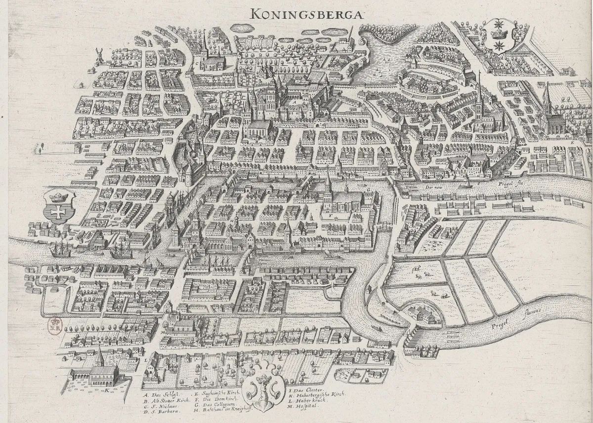
An Euler tour is a closed walk traversing every edge exactly once, and a graph admitting one is Eulerian. Note the word walk: vertices may be revisited freely, and only edges are rationed.[8]
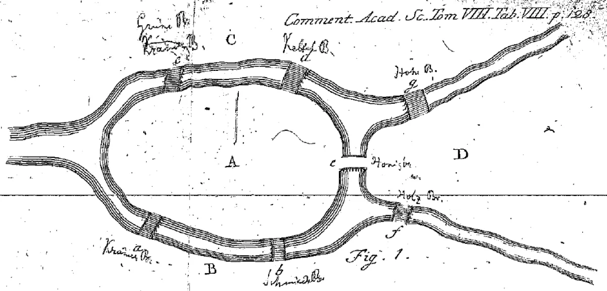
Before you read Euler's answer, try the walk. The map below is the 1736 city, and the seven bridges carry the names Königsberg gave them. Click a landmass to stand on it, then click bridges to cross them, one at a time and each one only once. After two failed attempts the map offers to show you what keeps going wrong.
A connected graph has an Euler tour if and only if every vertex has even degree.[8]
Every visit to a place uses one way in and one way out, so a place with an odd number of connections eventually strands you, and even the starting point must balance because you return to it. What is remarkable is that this obviously necessary local condition is also sufficient: a parity check at each vertex settles a global question about traversing the whole network.
Even degrees alone are not enough: two disjoint triangles have every degree equal to 2 and no Euler tour, so the theorem needs connectedness too. And an Euler tour is not a cycle, since it may revisit vertices. Visiting every vertex once is a different problem, the Hamilton cycle of Chapter 10.
Two applications, one obvious and one surprising. A mail carrier or snow plough must cover every street and return to the depot with least total travel. If every intersection has even degree an Euler tour solves it exactly; if not, choosing which streets to repeat is a minimum-weight matching problem on the odd-degree intersections. Edmonds and Johnson welded Euler's characterization to matching theory to give a polynomial-time algorithm for this route-inspection problem.[16] The surprise is genomics. Sequencers emit billions of short overlapping fragments, and making each fragment a vertex turns assembly into a Hamiltonian problem, intractable at that scale. Compeau, Pevzner and Tesler explain the fix: chop the fragments up and make the pieces the edges of a de Bruijn graph, so assembly becomes an Eulerian path problem, solvable efficiently.[17]
Suppose one extra bridge is built in Figure 1.21, joining the north bank \(N\) directly to the south bank \(S\). Can a walk now cross every bridge exactly once and finish where it began?
The adjacency and incidence matrices, cycle space and cut space
The edge space \(\mathcal{E}(G)\) is the collection of all subsets of \(E\), treated as vectors, where adding two edge sets keeps exactly the edges in one of them but not both (symmetric difference). The zero vector is the empty set, and every set is its own negative, since \(F + F = \emptyset\). The vertex space \(\mathcal{V}(G)\) is the same on subsets of \(V\); the dimensions are \(\|G\|\) and \(|G|\).[9]
All of this is arithmetic modulo 2, in the two-element field \(\mathbb{F}_2\) where \(1 + 1 = 0\). Think of each edge as carrying a switch: adding a set of edges flips those switches, and flipping twice returns you to the start, which is the rule \(F + F = \emptyset\).
The edge space also carries an inner product: \(\langle F, F' \rangle\) is 0 when the two sets share an even number of edges and 1 when odd. For a subspace \(\mathcal{F}\), the orthogonal complement \(\mathcal{F}^{\perp}\) is everything meeting every member of \(\mathcal{F}\) evenly, and \(\dim \mathcal{F} + \dim \mathcal{F}^{\perp} = \|G\|\).
The cycle space \(\mathcal{C}(G)\) is the subspace of \(\mathcal{E}(G)\) spanned by the edge sets of the cycles of \(G\). An edge set is a cut if it is all the edges crossing a split of \(V\) into two non-empty parts, and a bond is a minimal non-empty cut, one with no smaller cut inside it. The cut space \(\mathcal{B}(G)\) is all cuts plus the empty set.[9]
For an edge set \(D\), these say the same thing: \(D\) belongs to \(\mathcal{C}(G)\); \(D\) is a union of edge sets of cycles sharing no edges; every vertex of \((V, D)\) has even degree.[9]
Keep working with Figure 1.23. Choose the spanning tree \(T = \{ab, bc, cd\}\), whose chords are \(da\) and \(ac\). Adding \(da\) closes \(C_{da} = Q\), the square; adding \(ac\) closes \(C_{ac} = T_1\), the violet triangle. Those two form a basis, and \(T_2 = Q + T_1\). Now remove the tree edge \(bc\): the tree splits into \(\{a,b\}\) and \(\{c,d\}\), with crossing edges \(bc\), \(ac\), \(ad\), so \(D_{bc} = \{bc, ac, ad\}\). Test the duality below: \(Q\) and \(D_{bc}\) share exactly \(bc\) and \(ad\), an even number, so their inner product is 0.
Cuts assemble from the simplest ones. The atomic cut \(E(v)\) is the bundle of all edges at one vertex, and Proposition 1.9.2 says the cuts form a subspace generated by these: the cut with sides \(V_1\) and \(V_2\) is the sum of \(E(v)\) over \(v \in V_1\), since edges inside \(V_1\) are counted twice and cancel. Lemma 1.9.3 adds that every cut splits into bonds.[9]
\(\mathcal{C}(G) = \mathcal{B}(G)^{\perp}\) and \(\mathcal{B}(G) = \mathcal{C}(G)^{\perp}\): an edge set is a sum of cycles exactly when it meets every cut evenly, and a sum of cuts exactly when it meets every cycle evenly.[9]
Proof idea. Half of it is one observation: walk around a cycle and count how often you cross a given split of the vertices; you end where you began, so you crossed evenly. An edge set outside the cycle space has a vertex of odd degree, so it meets the atomic cut there oddly. The subtle step is the last: given \(F\) meeting every cycle evenly, contract every edge not in \(F\); the result has no odd cycle, so it splits into two camps, and pulling that split back exhibits \(F\) as a cut.
Let \(G\) be connected with \(n\) vertices, \(m\) edges and a spanning tree \(T\). The fundamental cuts \(D_f\), one per tree edge, form a basis of \(\mathcal{B}(G)\); the fundamental cycles \(C_e\), one per chord, form a basis of \(\mathcal{C}(G)\). Hence \(\dim \mathcal{B}(G) = n-1\) and \(\dim \mathcal{C}(G) = m - n + 1\).[9]
Proof idea. Independence is immediate, since the chord \(e\) appears in \(C_e\) and no other fundamental cycle. For spanning, add to any cycle \(C\) the fundamental cycle of each of its chords: the result lies in the cycle space but uses only tree edges, and the only such element is the empty set. The dimensions follow from the tree edge count \(n-1\), and \(m - n + 1\) is called the cyclomatic number.
Finally, the matrices. The incidence matrix \(B\) has one row per vertex and one column per edge, with a 1 wherever the vertex lies on the edge. The adjacency matrix \(A\) has a 1 wherever two vertices are joined, and its row sums are the degrees. The degree matrix \(D\) lists the degrees down its diagonal. Over \(\mathbb{F}_2\), \(B\) sends an edge set to the vertices meeting an odd number of its edges and \(B^{\top}\) sends a vertex set \(U\) to the edges with one end in \(U\), so the kernel of \(B\) is the cycle space and the image of \(B^{\top}\) is the cut space.[9] Over the real numbers \(BB^{\top} = A + D\), and with directions on the edges it becomes \(D - A\), the Laplacian behind spectral graph theory, spectral clustering and graph neural networks.
Orthogonal does not mean disjoint here. It means the two sets overlap in an even number of edges, which is why a non-empty set of even size is orthogonal to itself. Second, a cut is not any set of edges whose removal disconnects the graph: it is all the edges crossing a two-way split. A minimal non-empty cut is a bond.
Cuts are how computer vision separates an object from its background. Build a graph with one vertex per pixel and edges between neighbouring pixels weighted by how similar they look, then add two special vertices, one for "object" and one for "background": a cheapest cut separating those two traces the object boundary. Boykov and Funka-Lea show that these cuts reach global optima efficiently in any number of dimensions, including medical scans.[18] The duality that makes it computable is the subject of Chapter 6.
An edge set \(D\) belongs to the cycle space \(\mathcal{C}(G)\) exactly when which condition holds?
An edge set \(F\) contains exactly 4 edges. What is \(\langle F, F \rangle\)?
Other notions of graphs: directed, multigraphs, hypergraphs
A hypergraph is a pair \((V,E)\) where each edge is a non-empty subset of \(V\) of any size; ordinary graphs are the case where every edge has size 2. A directed graph, or digraph, sends each edge \(e\) to \(\operatorname{init}(e)\) and \(\operatorname{ter}(e)\), and points from the first to the second. Several edges may join one pair, parallel when they point the same way; an edge with \(\operatorname{init}(e) = \operatorname{ter}(e)\) is a loop. A multigraph keeps loops and repeated edges but forgets directions.[10]
An orientation chooses one of the two directions for each edge of an ordinary graph, and a digraph arising this way is an oriented graph. Flows in Chapter 6 and the tournament results in Chapter 10 live in that setting.
Multigraphs reuse most of the vocabulary, with three differences. Cycles of length 1 and 2 now exist, being a loop and a doubled edge. A loop contributes 2 to its vertex's degree, so degree and neighbour count stop agreeing, and it makes its vertex a cutvertex, so every 3-connected multigraph is an ordinary graph. Contraction gets simpler, since contracting \(e\) deletes no other edge. Plane duality in Chapter 4 and flows in Chapter 6 force multigraphs into the story anyway.[10]
One last note. Authors who take multigraphs as their default call the objects of this chapter simple graphs, so check which convention a paper uses before believing any degree count.
In a multigraph, what does a loop at the vertex \(v\) do to \(d(v)\)?
What to carry forward
Four things from this chapter appear on nearly every later page. First, the notation, which is why the table near the top exists and why ten other chapters link to it. Learn to read \(|G|\) and \(\|G\|\) apart, and remember that Diestel's indices ride high.
Second, the double-counting reflex: the degree-sum identity came from counting one set of pairs in two ways. Third, the extremal-choice reflex: take a longest path or a smallest counterexample, then ask what the extreme case cannot do. Proposition 1.3.1, Mader's theorem, Euler's theorem and the existence of normal spanning trees are all built that way.
Fourth, the shape of a good theorem. Euler's theorem reduces a global traversal question to a local parity check; the bipartite theorem reduces a two-camp question to one forbidden shape. Characterisations of that kind, where a property you cannot see is equivalent to one you can check, are what the rest of the book hunts, and Chapter 2 starts that hunt with matchings.
The chapter names two proof reflexes to carry forward. Which one produced the degree-sum identity \(\|G\| = \tfrac{1}{2}\sum_{v} d(v)\)?
Check your understanding
In Diestel's notation, what does \(\|G\|\) denote?
How many edges does the complete graph \(K^5\) have?
What does \(\delta(G)\) stand for?
How many vertices does the path \(P^4\) have?
Which of these guarantees that a graph is not bipartite?
A connected graph has 10 vertices and 9 edges. What must be true of it?
Which statement correctly characterizes a bridge?
For every non-trivial graph, which chain of inequalities always holds between the connectivity \(\kappa\), the edge-connectivity \(\lambda\), and the minimum degree \(\delta\)?
Which of these graphs has an Euler tour?
A connected graph has 6 vertices and 9 edges. What is the dimension of its cycle space \(\mathcal{C}(G)\)?
Sources and further reading
- R. Diestel, Graph Theory, 6th ed., Springer GTM 173 (2024), §1.1 (graphs, order and size, complete graphs \(K^n\), isomorphism, subgraphs and induced subgraphs, deletion and addition, join, complement, line graph).
- R. Diestel, Graph Theory, 6th ed., Springer GTM 173 (2024), §1.2 (neighbourhood and degree, \(\delta\), \(\Delta\), \(d(G)\), \(\varepsilon(G)\); the degree-sum identity; Proposition 1.2.1 on odd-degree vertices; Proposition 1.2.2 on dense subgraphs).
- R. Diestel, Graph Theory, 6th ed., Springer GTM 173 (2024), §1.3 (paths, cycles, girth, distance, diameter, radius, walks; Proposition 1.3.1; Proposition 1.3.2; Proposition 1.3.3; Theorem 1.3.4 of Alon, Hoory and Linial; Corollary 1.3.5).
- R. Diestel, Graph Theory, 6th ed., Springer GTM 173 (2024), §1.4 (components, separators, cutvertices, bridges, separations, \(\kappa\) and \(\lambda\); Proposition 1.4.1; Proposition 1.4.2; Theorem 1.4.3, Mader's theorem, 1972).
- R. Diestel, Graph Theory, 6th ed., Springer GTM 173 (2024), §1.5 (forests, trees, leaves, spanning trees, rooted trees and the tree-order, up- and down-closures, normal trees; Theorem 1.5.1; Corollary 1.5.2; Corollary 1.5.3; Lemma 1.5.4; Proposition 1.5.5).
- R. Diestel, Graph Theory, 6th ed., Springer GTM 173 (2024), §1.6 (\(r\)-partite and bipartite graphs, complete multipartite graphs, stars; Proposition 1.6.1 on odd cycles).
- R. Diestel, Graph Theory, 6th ed., Springer GTM 173 (2024), §1.7 (subdivisions \(TX\), topological minors, inflated graphs \(IX\), branch sets, minors \(X \preccurlyeq Y\), contraction \(G/e\); Proposition 1.7.1; Corollary 1.7.2; Proposition 1.7.3).
- R. Diestel, Graph Theory, 6th ed., Springer GTM 173 (2024), §1.8 (the Königsberg bridge problem; Theorem 1.8.1, Euler's tour theorem, 1736).
- R. Diestel, Graph Theory, 6th ed., Springer GTM 173 (2024), §1.9 (vertex and edge spaces over \(\mathbb{F}_2\), cycle space, cuts, bonds, cut space, fundamental cycles and cuts, incidence and adjacency matrices; Propositions 1.9.1, 1.9.2, 1.9.6, 1.9.7; Lemma 1.9.3; Theorems 1.9.4 and 1.9.5).
- R. Diestel, Graph Theory, 6th ed., Springer GTM 173 (2024), §1.10 (hypergraphs, directed graphs, orientations, multigraphs, suppressing a degree-2 vertex, the "simple graph" terminology note).
- D. J. Watts, S. H. Strogatz, "Collective dynamics of 'small-world' networks", Nature 393 (1998), 440–442. nature.com.
- R. Pastor-Satorras, A. Vespignani, "Epidemic spreading in scale-free networks", Physical Review Letters 86 (2001), 3200. arXiv:cond-mat/0010317.
- D. Gale, L. S. Shapley, "College Admissions and the Stability of Marriage", The American Mathematical Monthly 69(1) (1962), 9–15. Full text.
- National Resident Matching Program, "How the Matching Algorithm Works", official explainer. nrmp.org.
- A. E. Roth, E. Peranson, "The Redesign of the Matching Market for American Physicians: Some Engineering Aspects of Economic Design", American Economic Review 89(4) (1999), 748–780. aeaweb.org.
- J. Edmonds, E. L. Johnson, "Matching, Euler tours and the Chinese postman", Mathematical Programming 5 (1973), 88–124. springer.com.
- P. E. C. Compeau, P. A. Pevzner, G. Tesler, "How to apply de Bruijn graphs to genome assembly", Nature Biotechnology 29 (2011), 987–991. nature.com.
- Y. Boykov, G. Funka-Lea, "Graph Cuts and Efficient N-D Image Segmentation", International Journal of Computer Vision 70 (2006), 109–131. springer.com.
- T. Lengauer, Combinatorial Algorithms for Integrated Circuit Layout, Vieweg+Teubner (1990). springer.com.