Part II · The Classic Theory
Planar Graphs
Some networks can be drawn flat with no wires crossing; most cannot. After this chapter you will be able to count the faces of any flat drawing with Euler's formula, name the only two graphs that ever stand between a network and a crossing-free drawing, and turn loops into cuts with plane duality.
Three houses, three utilities
Here is a puzzle that has circulated for over a century. Three houses each need a connection to three utility stations: water, gas, and electricity. Nine supply lines in total. Can you route all nine lines on flat ground so that no two lines cross?
Try it. Every attempt ends with eight lines placed and the ninth trapped: wherever it goes, it must cross something. The puzzle is not asking for cleverness; it is asking for something impossible, and by the middle of this chapter you will be able to prove that in four lines of arithmetic.
In graph language the puzzle is a specific graph: three vertices on one side, three on the other, and all nine possible edges between the sides. This is the complete bipartite graph \(K_{3,3}\) (read it as "K three three"): two groups of three, every cross-pair joined, no edges inside a group. The puzzle asks whether \(K_{3,3}\) can be drawn in the plane so that edges meet only at their shared endpoints. Graphs that can be drawn that way are called planar, and this whole chapter, following Chapter 4 of Diestel's book[2], is about them.
The chapter builds up four very different answers to the question "which graphs are planar?": a counting law (Euler's formula), a pair of forbidden patterns (Kuratowski's theorem), a statement in linear algebra (MacLane's theorem), and even a statement about orderings (Schnyder's theorem). The same class of graphs, described in the languages of geometry, combinatorics, algebra, and order theory. Along the way we will meet plane duality, the swap of vertices and faces that Chapter 5 will use for map colouring and Chapter 6 for flows.
The houses-and-utilities puzzle asks for a crossing-free drawing of which graph?
Plane or planar? A picture versus a possibility
The first distinction of the chapter is small but load-bearing, and mixing it up is the single most common beginner error. A plane graph is an actual picture: specific points in the plane serving as vertices, specific curves serving as edges, no two curves crossing. A planar graph is an abstract graph, a bare list of vertices and edges, which could be drawn as a plane graph. Plane is a property of a drawing; planar is a property of a graph.
Why does the difference matter? Because one abstract graph has many drawings, and a bad drawing proves nothing. Take \(K^4\), the complete graph on four vertices: four dots, all six pairs joined. (Diestel writes complete graphs as \(K^n\); many other books write \(K_n\). Same object.) Drawn as a square with both diagonals, \(K^4\) shows a crossing. Drawn as a triangle with the fourth vertex inside, it shows none. The first picture is not a plane graph; the second is; the abstract graph \(K^4\) is planar either way.
"My drawing has crossings, so the graph is not planar." No: planarity asks whether some crossing-free drawing exists, not whether the one in front of you is crossing-free. To show a graph is planar, exhibit one good drawing. To show it is not planar you need an argument that defeats every possible drawing, and finding such arguments is exactly what this chapter is for.
This raises a subtler question that Section 4.3 of the book takes seriously: if one graph has many drawings, when should two drawings count as "the same drawing"? Hold that thought; we first need faces and Euler's formula.
You draw a graph \(G\) and your picture has two crossings. What follows?
New notation in this chapter
Rows marked "reminder" were introduced in Chapter 1 and return here in a load-bearing role.
| Symbol | Read it as | Meaning | Tiny example |
|---|---|---|---|
| \(F(G)\) | "the faces of G" | The set of faces of a plane graph \(G\): the connected regions the drawing cuts the plane into, the unbounded outer region included. | A drawn triangle has \(|F(G)| = 2\): inside and outside. |
| \(\ell\) | "ell, the face count" | \(\ell = |F(G)|\), the number of faces; used alongside \(n = |V|\) and \(m = |E|\) in Euler's formula. | For the drawn cube: \(n=8\), \(m=12\), \(\ell=6\). |
| \(G[f]\) | "the boundary of f" | The subgraph of \(G\) whose points form the frontier of the face \(f\): what you touch walking the rim of \(f\). (Same brackets as induced subgraphs \(G[U]\); the argument tells you which is meant.) | In a square with one diagonal, each triangular face has a triangle as its boundary. |
| \(\mathring{e}\), \(\mathring{P}\) | "the interior of e" | An edge (or arc) with its two endpoints removed: just the open middle part. | If \(P\) runs from \(x\) to \(y\), then \(\mathring{P} = P \setminus \{x,y\}\). |
| \(S^2\) | "the sphere" | The surface of a ball. Drawings transfer between the plane and the sphere, where the outer face loses its special status. | Puncture a sphere-drawing inside any face; that face becomes the outer one. |
| \(K_{3,3}\) | "K three three" (reminder) | The complete bipartite graph: two groups of three vertices, all nine cross edges, none inside a group. | The houses-and-utilities graph. |
| \(TX\) | "a subdivision of X" (reminder) | The graph \(X\) with edges replaced by paths through new in-between vertices; \(G \supseteq TX\) means \(G\) contains such a stretched copy of \(X\) as a subgraph. | Replacing edge \(xy\) by the path \(x\,v\,y\) gives a \(TX\). |
| \(\mathcal{C}(G)\) | "the cycle space of G" (reminder) | The vector space over the two-element field whose vectors are edge sets of even-degree subgraphs; spanned by edge sets of cycles, with addition = symmetric difference. | Two triangle faces of a drawn square-with-diagonal sum to the outer square. |
| \(G^*\) | "G star, the dual of G" | The plane dual: one new vertex inside each face of \(G\), one new edge crossing each edge of \(G\). | The dual of the drawn cube is the octahedron. |
| \(e^*\) | "e star, the dual edge" | The edge of \(G^*\) that crosses \(e\), joining the dual vertices of the two faces on either side of \(e\); a loop if both sides are the same face. | A bridge in \(G\) dualizes to a loop in \(G^*\). |
| \(v^*(f)\), \(f^*(v)\) | "the dual vertex of f", "the dual face of v" | The vertex of \(G^*\) placed inside face \(f\); the face of \(G^*\) containing vertex \(v\). Two bijections that make duality tight. | The outer face of a drawn triangle contributes one dual vertex outside the triangle. |
The table reads \(TX\) as "a subdivision of \(X\)". What is such a subdivision?
A small toolkit from the geometry of the plane
Before graphs can live in the plane, we need a few honest facts about the plane itself. Diestel collects them in Section 4.1[1], states them precisely, and does not prove them, because the proofs are topology, not graph theory. We follow suit.
A straight line segment is the straight stretch between two points, endpoints included. A polygon is a closed loop built from finitely many straight segments that never touches itself. A polygonal arc, called simply an arc in this chapter, is a non-self-touching chain of finitely many straight segments running from one point (an endpoint) to another; the arc links its two endpoints. The interior \(\mathring{P}\) of an arc \(P\) is the arc minus its two endpoints.
Why only piecewise-straight curves? Because any crossing-free drawing can be straightened into one, and restricting to them keeps every topological statement elementary. Nothing is lost and much wildness is avoided.
Two more notions. For an open set \(O\) of the plane, a region of \(O\) is a maximal connected chunk: a set of points of \(O\) any two of which can be linked by an arc staying inside \(O\). The frontier of a set \(X\) is its boundary line: all points \(y\) such that every small disc around \(y\) meets both \(X\) and the rest of the plane. The frontier of an open disc, for example, is its bounding circle. One notational care: Diestel keeps \(\setminus\) for differences of point sets in the plane (so \(\mathbb{R}^2 \setminus G\) is "the plane minus the drawing") and the minus sign for graph deletion (so \(G - e\) is "the graph with edge \(e\) removed").
The engine behind everything else is a statement so obvious-sounding that its actual content is easy to miss.
For every polygon \(P\) in the plane, the set \(\mathbb{R}^2 \setminus P\) has exactly two regions, one bounded and one unbounded, and each of the two has the entire polygon \(P\) as its frontier.[1]
In words: a closed non-self-crossing loop cuts the plane into exactly an inside and an outside, and the loop is the complete border of both. Nearly every proof in this chapter reduces at some point to "this point is inside, that point is outside, so any arc between them must cross the loop." Two companion facts get used just as often. First, three arcs sharing both endpoints but otherwise disjoint carve the plane into exactly three regions, and any arc through the middle region between points of the two outer arcs must cross the middle arc (Lemma 4.1.2). Second, an arc drawn across a region does not split that region if it merely hangs there connecting two blobs of the frontier (Lemma 4.1.3): arcs, unlike polygons, do not separate. Cycles enclose; paths do not.
One face of every drawing is infinite, which feels awkward: why should one face be special? The fix is to draw on a sphere instead. A standard map projection (stereographic projection: put a sphere on the plane, project from the north pole) converts any flat drawing into a sphere drawing and back. On the sphere all faces are ordinary bounded patches; which one becomes the "outer" face is just an accident of where the north pole sits. Whenever a theorem seems to treat the outer face specially, mentally re-inflate the sphere: the special status evaporates, and any face can be rotated into being the outer one.
A polygon and a polygonal arc are each drawn in the plane. Which of the two cuts the plane into two regions?
Plane graphs and their faces
Now the main object, with all its fine print.
A plane graph is a pair \((V, E)\) of finite sets where: (i) the vertices \(V\) are points of the plane; (ii) every edge is an arc linking two vertices; (iii) different edges have different sets of endpoints; and (iv) the interior of an edge contains no vertex and no point of any other edge. Plainly: an actual crossing-free picture. Each clause bans one kind of mess: no doubled edges, no edge passing through a vertex, no two edges overlapping or crossing.
A plane graph is simultaneously a picture and a graph: the same letter \(G\) names the abstract graph and the set of points of the plane covered by the drawing. That double life is deliberate, and the point-set reading is what makes the next definition work.
A face of a plane graph \(G\) is a region of \(\mathbb{R}^2 \setminus G\): a maximal connected piece of the plane left over when the drawing is removed. The set of faces is \(F(G)\). Exactly one face is unbounded, the outer face; the others are inner faces. The boundary of a face \(f\), written \(G[f]\), is the subgraph of \(G\) whose points form the frontier of \(f\); the face is incident with the vertices and edges of its boundary.
That the boundary of a face really is a subgraph, never half an edge, is a theorem, not part of the definition. The key local fact (Diestel's Lemma 4.2.2[2]) says three things. If the frontier of a face contains any interior point of an edge \(e\), it contains all of \(e\). If \(e\) lies on a cycle, then \(e\) borders exactly two faces. And if \(e\) lies on no cycle, it borders exactly one. The proof idea is pleasantly local: around any interior point of \(e\), take a disc so small it meets the drawing only in \(e\); the disc is cut into two half-discs, each sitting inside some face, so at most two faces touch \(e\) there. If \(e\) lies on a cycle, the Jordan curve theorem puts the two half-discs on opposite sides of that cycle, in different faces: a cycle edge is a wall between two rooms. If \(e\) is a bridge, the arc-does-not-separate lemma says both half-discs belong to one face: a bridge is a wall jutting into the middle of a single room.
Several structural facts now fall out, each one a small step toward Euler's formula and Whitney's theorem.
Forests enclose nothing. A plane forest (a drawing of a cycle-free graph) has exactly one face (Proposition 4.2.4): with no cycles there are no walls that close, so no territory ever gets enclosed. This will be the base case of Euler's formula.
Only a cycle has two rooms with the same wall. If two distinct faces have exactly the same boundary, the whole graph is just a cycle (Lemma 4.2.5). In every richer graph, a face is pinned down by its boundary; this uniqueness matters when we later match up faces of different drawings.
In 2-connected graphs, faces are bounded by cycles. Recall from Chapter 3 that a graph is 2-connected when it is connected, has at least three vertices, and stays connected after deleting any one vertex; such graphs are built by starting from a cycle and repeatedly gluing on paths. Each glued path lands inside some face and splits it into two, and both new faces inherit cycle boundaries. Hence every face of a 2-connected plane graph is bounded by a cycle (Proposition 4.2.6).
In 3-connected graphs, you can spot the face boundaries without looking at the picture. This is the quiet star of the chapter (Proposition 4.2.7): in a 3-connected plane graph (deleting any two vertices leaves it connected), the face boundaries are precisely the non-separating induced cycles, that is, the cycles with no chord whose deletion leaves the rest of the graph connected. Both properties are purely combinatorial: they mention no drawing. One direction: a chordless cycle that separates nothing can have graph-stuff on only one of its two sides, by the Jordan curve theorem, so its other side is a bare face. The other direction: a face boundary cannot have a chord (the chord and a connecting path would be forced to cross) and cannot separate the graph (Menger's theorem from Chapter 3 supplies three independent paths, one of which dodges the face entirely). Keep this in your pocket: it is the whole proof of Whitney's uniqueness theorem below.
A plane graph is maximally plane if no new edge can be added between its existing vertices while keeping the picture a plane graph: the drawing is full. A plane graph is a plane triangulation if every face, the outer face included, is bounded by a triangle.
For at least three vertices, these two conditions coincide (Proposition 4.2.8): a picture is full exactly when every room, the infinite one included, is triangular. One direction is immediate: in a triangular room, all three boundary vertices are already pairwise adjacent, so no new edge fits. The converse takes the Jordan machinery: a bigger room always leaves space for a chord.
Forgetting that the outer face counts. A drawn square with one diagonal is not a plane triangulation: its two inner faces are triangles, but the outer face is bounded by a 4-cycle. The same oversight makes people compute \(n - m + \ell = 1\) and conclude that Euler's formula failed. The unbounded region is a face, always.
In a plane graph, an edge \(e\) lies on no cycle. How many faces is \(e\) incident with?
Which of these plane drawings is a plane triangulation?
Euler's formula: one law that rules every drawing
Now a theorem of 1752, and still the only purely quantitative law of planarity.
If a connected plane graph has \(n\) vertices, \(m\) edges and \(\ell\) faces, then \[ n - m + \ell = 2. \] Read it aloud: vertices, minus edges, plus faces, equals two. Always. No matter how the graph is drawn.[2]
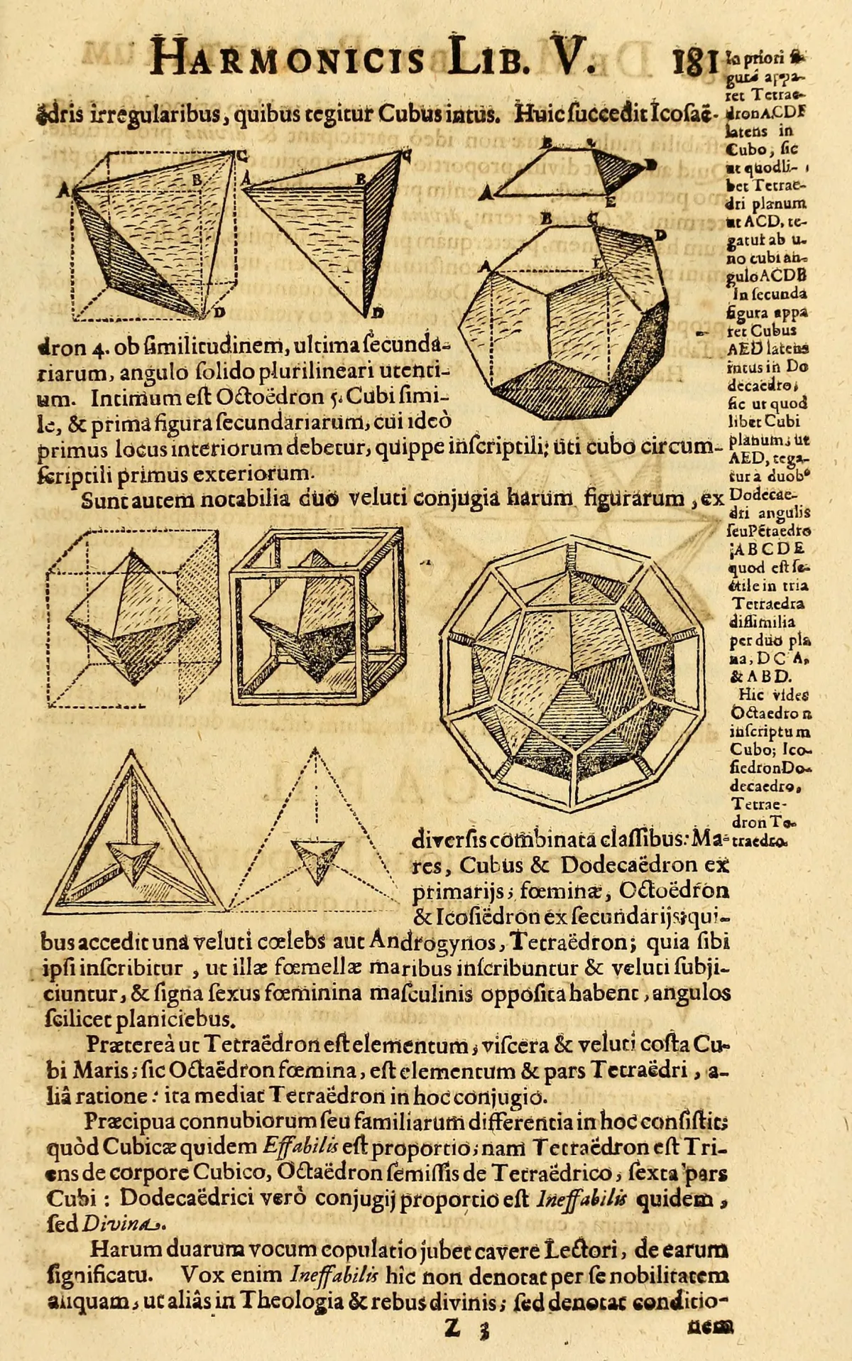
Pause on what is being claimed. The number of faces is a property of a particular picture, yet the formula says the picture does not matter: \(\ell = 2 - n + m\) is decided by the abstract graph alone. Every drawing of a given connected planar graph has the same number of faces.
The cube graph: 8 corners, 12 edges. Drawn flat as a small square inside a large one (Figure 4.3), it shows four trapezoid faces, the inner square, and the outer face: \(\ell = 6\). Check: \(8 - 12 + 6 = 2\). And 6 is exactly what the formula predicts from the abstract data alone: \(\ell = 2 - 8 + 12 = 6\). Any other crossing-free drawing of the cube must also produce six faces.
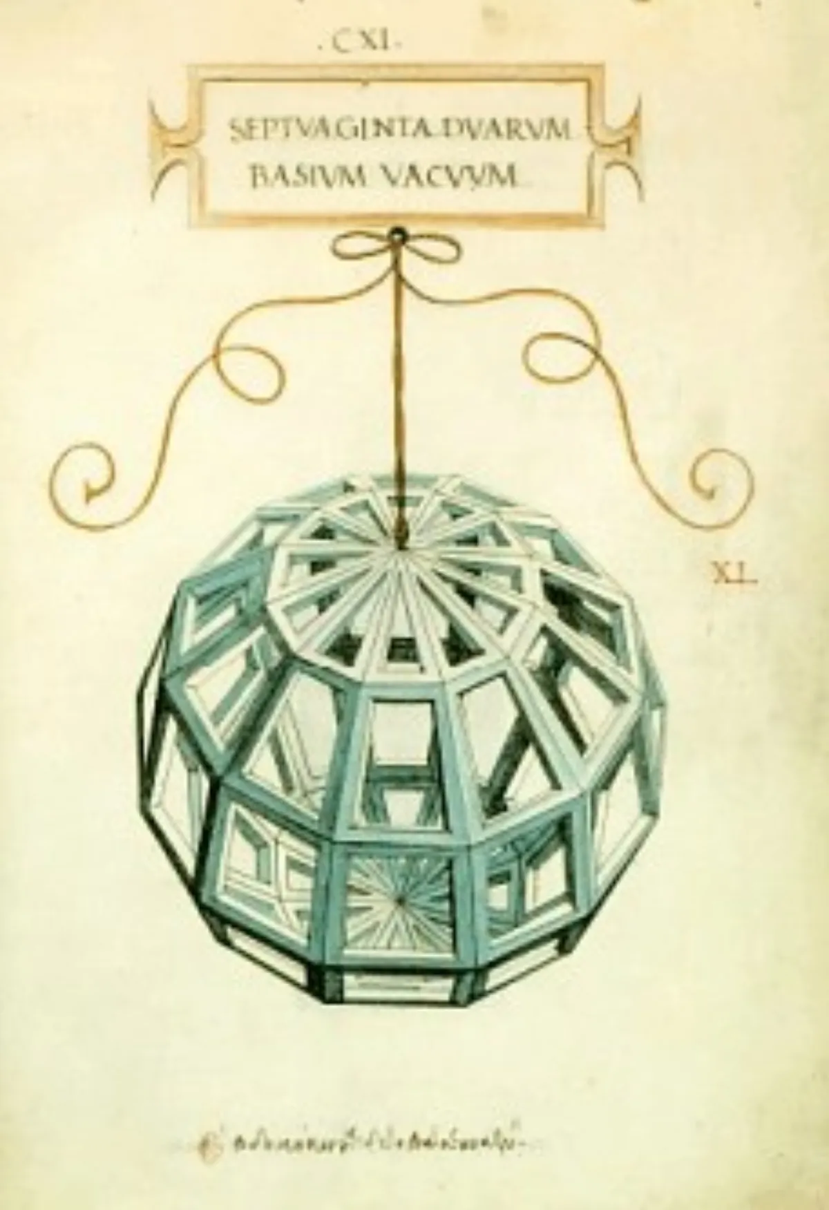
The proof idea is an induction on the number of edges, with \(n\) fixed. If the connected graph has no cycle, it is a tree: \(m = n - 1\) edges (from Chapter 1) and, since forests enclose nothing, one face; the sum is \(n - (n-1) + 1 = 2\). Otherwise pick an edge lying on a cycle and delete it. That edge was a wall between two distinct rooms; deleting it merges them into one. So \(m\) drops by one, \(\ell\) drops by one, and the alternating sum \(n - m + \ell\) does not move. Walk the induction down to a tree and you are done. The careful bookkeeping ("exactly two faces merge into exactly one") is precisely the wall-between-two-rooms fact from the previous section.
From one line of arithmetic, an avalanche of consequences.
A planar graph with \(n \ge 3\) vertices has at most \(3n - 6\) edges, with equality exactly for the graphs whose drawings are plane triangulations.[2]
Proof idea: count edge-face incidences twice. Every face is bounded by at least 3 edges; every edge borders at most 2 faces; therefore \(3\ell \le 2m\), in words: three times the faces is at most twice the edges. Substitute \(\ell \le \tfrac{2}{3}m\) into Euler's formula and solve: \(m \le 3n - 6\). The striking consequence: planar graphs are sparse. However enormous, a planar graph averages fewer than six edge-ends per vertex, so it always has a vertex of degree at most 5, a fact Chapter 5 will lean on for colouring.
And the bound draws blood immediately. Consider \(K^5\), the complete graph on five vertices: \(n = 5\) allows at most \(3 \cdot 5 - 6 = 9\) edges, but \(K^5\) has \(\binom{5}{2} = 10\). One edge over budget. No drawing exists.
What about the utilities graph? \(K_{3,3}\) has \(n = 6\) and \(m = 9\), comfortably under \(3 \cdot 6 - 6 = 12\), so the plain bound says nothing. But \(K_{3,3}\) is bipartite, so it contains no triangle: its shortest cycles have length 4. Rerun the double count with rooms of at least 4 walls: \(4\ell \le 2m\), which with Euler gives \(m \le 2n - 4\) for triangle-free planar graphs. For \(K_{3,3}\) that allows at most \(2 \cdot 6 - 4 = 8\) edges. It has 9. The houses cannot be wired, and that is the whole proof.
One step further, at no extra cost. Subdividing an edge (replacing it by a path through new vertices) clearly cannot rescue planarity: a drawing of the subdivided graph would yield a drawing of the original by ignoring the new dots along the way. So no plane graph contains a subdivision \(TK^5\) or \(TK_{3,3}\), a stretched copy of either culprit, as a subgraph (Corollary 4.2.11). This is the easy half of Kuratowski's theorem. The astonishing half, that these two are the only obstacles, comes two sections from now.
"My graph has fewer than \(3n - 6\) edges, so it is planar." The bound is one-way traffic: too many edges disproves planarity, but few edges prove nothing. \(K_{3,3}\) sits well under the bound and is not planar; a huge sparse graph can hide a stretched \(K^5\) deep inside. Also mind the fine print: the bound needs \(n \ge 3\), the triangle-free refinement needs bipartite-style girth, and Euler's formula as stated needs the graph connected.
What is the largest number of edges in a planar graph with 10 vertices? Answer: \(3 \cdot 10 - 6 = 24\). And the bound is tight only for triangulations, so any planar graph achieving 24 edges on 10 vertices must, in every drawing, have all faces (outer included) bounded by triangles. Sparser targets are just as quick: a triangle-free planar graph on 10 vertices stops at \(2 \cdot 10 - 4 = 16\) edges.
A classic exercise in Diestel's chapter: a football (soccer ball) is sewn from pentagons and hexagons, three panels meeting at every seam corner. Feed those facts into Euler's formula and the arithmetic forces the number of pentagons to be exactly 12, no matter how many hexagons there are.[7] The same arithmetic governs fullerenes, the closed carbon-cage molecules built from pentagonal and hexagonal rings: every one of them, whatever its size, has exactly twelve pentagonal rings. Euler's formula, disguised as chemistry.
Two people draw the same connected planar graph in different ways. One counts 7 faces, the other 8. What must be true?
A graph has \(n = 6\) vertices and \(m = 9\) edges, well under \(3n - 6 = 12\). What does the edge bound let you conclude?
When are two drawings the same drawing?
Back to the question we parked earlier. An abstract planar graph can be drawn in many ways. When should two drawings count as genuinely different, and when are they merely the same picture wiggled about? Diestel's Section 4.3[3] offers three answers of decreasing strictness, then shows they mostly collapse into one. (The book marks this section as skippable on a first pass; read it as the chapter's philosophical hinge, where topology hands over to combinatorics.)
First, the strictest: two plane graphs are topologically isomorphic if a continuous deformation of the whole sphere carries one drawing onto the other. (The sphere, not the plane, so that an inner face of one drawing is allowed to correspond to the outer face of the other; on the sphere the outer face is not special.) Second: they are combinatorially isomorphic if some isomorphism between the underlying graphs extends to their faces, matching face to face so that a vertex or edge lies on the boundary of a face exactly when its image lies on the boundary of the matching face. Third, and weakest: they are graph-theoretically isomorphic if an isomorphism maps the collection of face-bounding subgraphs of one drawing onto that of the other, without even tracking which subgraph bounds which face.
Theorem 4.3.1 collapses the ladder: the weakest notion already implies the middle one (the face matching reappears for free, uniquely unless the graph is a cycle, because faces are pinned down by their boundaries), and for 2-connected graphs the middle notion implies the strongest. The proof of that last step builds a sphere deformation piece by piece: match the vertices, then bend each edge onto its partner edge, then fill in each face using the Jordan–Schoenflies theorem, which extends a correspondence between two circles to the discs they bound. This is where 2-connectedness earns its keep: face boundaries are then genuine cycles, i.e. circles, exactly what the filling theorem needs.
So for 2-connected graphs, "same face structure" and "deformable into each other" are one notion, and we simply call two embeddings of the same graph equivalent when the canonical correspondence between the two drawings is such an isomorphism. Can inequivalent drawings actually happen? Yes, easily, once the graph has weak points:
The appendages in Figure 4.6 can be flipped into different faces because a single vertex, \(x\), is the only anchor holding them. 3-connectedness removes exactly this freedom, and then something remarkable happens:
Any two planar embeddings of a 3-connected graph are equivalent. In plain terms: a 3-connected planar graph has essentially one drawing.[3]
The proof is three lines, because all the work is already done. By Theorem 4.3.1 it suffices to check the weakest condition: that face-bounding cycles map to face-bounding cycles. But in a 3-connected plane graph, "bounds a face" means "is a non-separating induced cycle", and that is an abstract property of the graph, preserved by every isomorphism. Done. The drawing was never a free choice; it was encoded in the abstract graph all along.
Diestel's chapter notes point to Steinitz's theorem: the 3-connected planar graphs are exactly the corner-and-edge skeletons of 3-dimensional convex polyhedra.[7] Whitney's unique-drawing theorem is the combinatorial shadow of a polyhedron's rigidity of shape, and Euler's \(n - m + \ell = 2\) is literally the polyhedron formula (corners minus edges plus faces) that gets checked on cubes and pyramids in school. The cube: \(8 - 12 + 6 = 2\). A pyramid with a square base: \(5 - 8 + 5 = 2\).
Figure 4.6 shows one graph with two drawings that are not equivalent. Which feature of the graph makes that possible?
Kuratowski's theorem: exactly two obstacles
We know two culprits: no planar graph contains a stretched \(K^5\) or a stretched \(K_{3,3}\). Kuratowski's theorem is the converse, and it deserves a moment of awe before the details: among all the infinitely many graphs, exactly two are responsible for every failure of planarity, ever. Any non-planar graph, however enormous, contains a stretched copy of one of them.
Two containment notions from Chapter 1 need re-glossing, because the theorem uses both. \(G\) contains \(X\) as a topological minor if \(G\) has a subgraph that is a subdivision \(TX\): a copy of \(X\) whose edges have been stretched into paths through new in-between vertices. \(G\) contains \(X\) as a minor if \(X\) can be obtained from a subgraph of \(G\) by contracting connected chunks of vertices into single points. Minor containment is the more generous notion: every topological minor is a minor, but not conversely. For our two culprits, however, the notions coincide (Lemma 4.4.2): a graph has a \(K^5\) or \(K_{3,3}\) minor if and only if it has one of them as a topological minor. The reason, in brief: \(K_{3,3}\) has maximum degree 3, and minors of maximum degree at most 3 are automatically topological (a Chapter 1 fact); and a smallest possible \(K^5\) minor either has star-shaped branch chunks, making it a genuine \(TK^5\), or hides a \(K_{3,3}\) minor inside instead.
For any graph \(G\), the following are equivalent: (i) \(G\) is planar; (ii) \(G\) has no \(K^5\) and no \(K_{3,3}\) minor; (iii) \(G\) contains no \(TK^5\) and no \(TK_{3,3}\) as a subgraph.[4]
The proof runs through 3-connectedness, and its heart is a drawing argument worth seeing (Lemma 4.4.3): every 3-connected graph without a \(K^5\) or \(K_{3,3}\) minor is planar. Induct on the number of vertices. Chapter 3 supplies the crucial tool: every 3-connected graph on more than four vertices has an edge \(xy\) whose contraction (merging \(x\) and \(y\) into one vertex) leaves it 3-connected. Contract it; the smaller graph has no forbidden minor either, so by induction it has a drawing. Now delete the merged vertex from that drawing. It sat inside some face of the rest, and since the rest is 2-connected, that face is bounded by a cycle \(C\), with all the former neighbours of \(x\) and of \(y\) sitting on \(C\). Re-read the drawing as a drawing of \(G - y\) with \(x\) at the merged position. It remains to place \(y\). The neighbours of \(x\) chop \(C\) into arcs. If all of \(y\)'s neighbours happen to lie on a single one of those arcs, there is a free pocket beside that arc, and \(y\) drops in with room to spare (Figure 4.8). If not, a short case analysis shows the graph was guilty all along: two of \(y\)'s neighbours interleaved around \(C\) with two of \(x\)'s produce a \(TK_{3,3}\), and \(x\), \(y\) sharing three neighbours on \(C\) produces a \(TK^5\). Contradiction, so the good case is the only case.
The general case then reduces to the 3-connected one by a purely combinatorial argument (Lemmas 4.4.4 and 4.4.5): take a graph with as many edges as possible subject to containing no \(TK^5\) or \(TK_{3,3}\); such an edge-maximal graph, it turns out, is automatically 3-connected once it has at least four vertices. Pumping a Kuratowski-free graph full of edges welds it together. So the 3-connected case was the general case in disguise, and the theorem follows. (Diestel states Lemma 4.4.4 in more generality than needed here, on purpose: Chapter 7 reuses it for extremal problems.)
Three tidy consequences round off the section. First (Proposition 4.4.1): a maximal plane graph, one whose particular drawing is full, is always maximally planar, meaning no edge can be added in any drawing. You can never get stuck by drawing badly. Second, also 4.4.1: a planar graph with \(n \ge 3\) vertices is maximally planar exactly when it has exactly \(3n - 6\) edges; the extremal count is drawing-independent. Third (Corollary 4.4.7): every maximal planar graph with at least four vertices is 3-connected, so by Whitney it has essentially one drawing. Triangulations are the rigid skeletons of the planar world.
Hunting for \(K^5\) or \(K_{3,3}\) as literal subgraphs. The obstruction is a subdivision or minor: the five branch vertices of a \(TK^5\) may be joined by long winding paths rather than direct edges. The Petersen graph (a famous 10-vertex, 3-regular graph) contains no \(K^5\) subgraph at all, yet it is non-planar: it contains \(K^5\) as a minor. Looking only for literal copies misses almost every non-planar graph.
Wires etched on one layer of a printed circuit board cannot cross. So a circuit whose connection graph is planar can, in principle, be wired on a single layer, and non-planarity is exactly what forces multi-layer boards and "vias", the little vertical connections between layers. In chip design (very-large-scale integration, VLSI), crossing minimization and the extraction of large planar subgraphs are genuine engineering objectives, and planarity theory explains the cost structure of the whole layout problem: why crossings are expensive and why layers exist. The standard reference on the graph algorithmics of circuit layout is Lengauer's monograph.[8] Planarity testing itself is efficient: algorithms exist that either output a crossing-free drawing or point at the offending Kuratowski configuration, so the theorem doubles as a practical certificate of impossibility.
The Petersen graph contains no \(K^5\) subgraph, yet it is not planar. Why is that no contradiction?
Planarity without pictures: algebra and order
Everything so far has been geometric. Diestel's Section 4.5[5] presents two characterizations of planarity in which no drawing appears at all, and they are among the strangest facts in the book.
Recall the cycle space from Chapter 1: \(\mathcal{C}(G)\), the vector space over the two-element field whose vectors are edge sets, spanned by the edge sets of cycles, where adding two edge sets means taking their symmetric difference (keep the edges in exactly one of the two sets). Its dimension is \(m - n + 1\) for a connected graph: edges, minus vertices, plus one.
A family of edge sets is sparse if every edge of the graph lies in at most two members of the family. Plainly: no edge is overworked.
A graph is planar if and only if its cycle space has a sparse basis: a spanning set of independent cycles in which no edge appears more than twice.[5]
Where would such a basis come from? From the faces, of course. In a 2-connected plane graph, the boundaries of the inner faces are cycles, they generate the whole cycle space (the inner face boundaries lying inside any cycle sum to that cycle, because shared interior edges cancel in pairs), and each edge borders at most two faces, so no edge lies in more than two of them. Drawing a graph hands you a sparse basis for free. Figure 4.9 shows the smallest interesting case.
The converse direction is where it gets clever. Sparse bases survive edge deletion (delete an edge and drop, or merge, the one or two basis cycles that used it), so it is enough to show that the two Kuratowski graphs have no sparse basis; then any graph with a sparse basis avoids them as topological minors, and Kuratowski's theorem finishes the job. And the culprits fail by bare counting. For \(K^5\): the cycle space has dimension \(10 - 5 + 1 = 6\); take a supposed sparse basis of 6 cycles, add to the list the sum of all 6; now 7 nonempty edge sets, each a cycle-like set of at least 3 edges, need at least 21 edge-slots, but sparseness plus the extra set caps the total at twice the number of edges, \(2 \cdot 10 = 20\). For \(K_{3,3}\): dimension \(9 - 6 + 1 = 4\); shortest cycles have length 4 (its girth); five sets of size at least 4 need 20 slots, but only \(2 \cdot 9 = 18\) exist. Planarity, decided by linear algebra.
A cousin of MacLane's criterion, for 3-connected graphs, is Kelmans' theorem (1978, often called Tutte's planarity criterion; Diestel 4.5.2): a 3-connected graph is planar if and only if every edge lies on at most (equivalently, exactly) two non-separating induced cycles.[5] The forward direction you already believe: those cycles are exactly the face boundaries, and every edge is a wall between exactly two rooms. The backward direction is two big theorems shaking hands: Tutte's theorem from Chapter 3 says the non-separating induced cycles generate the whole cycle space of a 3-connected graph, and if each edge lies on at most two of them, that generating family contains a sparse basis, so MacLane applies. Count chordless cycles, conclude drawability.
The last characterization is the strangest, and Diestel states it without proof.
The incidence poset of a graph \(G\) is the partially ordered set on \(V \cup E\) in which \(v < e\) exactly when the vertex \(v\) is an endpoint of the edge \(e\), and nothing else is comparable. (For a single edge \(xy\): the poset says \(x < xy\) and \(y < xy\), and \(x, y\) are incomparable.) A linear extension of a partial order is a total order that agrees with it: one legal way to line everything up. The dimension of a poset is the least number of linear extensions whose intersection is exactly the given order: enough rankings that every incomparable pair gets ordered both ways somewhere.
A graph is planar if and only if the dimension of its incidence poset is at most 3.[5]
Sit with that. Form the humblest possible order, "this vertex is an endpoint of this edge", and ask how many total orderings are needed to pin it down. Three or fewer: planar. Four or more: not planar. No topology, no algebra, no drawing; pure order theory detects exactly the graphs that can be drawn flat. Beyond the book, the technique behind Schnyder's proof also yields straight-line drawings of planar graphs on small grids, which is why it shows up inside practical graph-layout software.
Why does a plane drawing of a 2-connected graph hand you a sparse basis of its cycle space for free?
\(K_{3,3}\) is not planar. What does Schnyder's criterion therefore say about its incidence poset?
Plane duality: swapping vertices and faces
The chapter closes with its most elegant construction. Look at any map: countries, borders, and corner points where borders meet. Now put a capital city inside each country and join capitals of neighbouring countries by a road crossing their shared border. The map of capitals and roads is a new graph, born from the faces of the old one. That is plane duality.
One technicality first. The dual construction produces loops (an edge from a vertex back to itself) and parallel edges (several edges with the same two endpoints), which our definition of plane graphs banned. So Diestel widens the frame[6]: a plane multigraph is like a plane graph except that an edge may also be a closed loop (a polygon touching exactly one vertex), and distinct edges may share both endpoints. Loops and parallel pairs count as cycles. Without this generality the theory collapses; you will see why in Figure 4.10.
Given a connected plane multigraph \(G\), its plane dual \(G^*\) is built by three moves: place one new vertex \(v^*(f)\) inside each face \(f\) of \(G\); for each edge \(e\) of \(G\), draw one new edge \(e^*\) crossing \(e\) exactly once and touching \(G\) nowhere else, joining the dual vertices of the two faces on either side of \(e\) (a loop, if the same face lies on both sides); and observe that each old vertex \(v\) ends up inside exactly one face \(f^*(v)\) of the new graph. Every connected plane multigraph has a dual, the dual is itself a connected plane multigraph, and \(G\) is in turn a dual of \(G^*\).
Vertex counts and face counts swap while the edge count stays put. The drawn cube (Figure 4.3) has 8 vertices, 12 edges, 6 faces; its dual, one vertex per face, is the octahedron: 6 vertices, 12 edges, 8 faces. Euler's formula is symmetric under the swap, as it must be.
Now the punchline the picture is hinting at. Recall from Chapter 1 that a cut is the set of edges running between the two sides of a vertex partition, and a bond is a minimal nonempty cut: a cut no proper nonempty part of which is itself a cut.
In a connected plane multigraph \(G\) with plane dual \(G^*\): an edge set \(E\) is the edge set of a cycle in \(G\) if and only if the corresponding dual edge set \(E^* = \{e^* : e \in E\}\) is a bond in \(G^*\).[6]
The proof idea is the Jordan curve theorem doing what it does best. A cycle in \(G\) splits the plane into inside and outside. Every face of \(G\) lies wholly in one or the other, so the dual vertices split into two camps, and the dual edges crossing the cycle are precisely the edges between the camps: a cut, and a minimal one, since walking between faces on the same side never crosses the cycle. Conversely, a dual bond traps a set of faces, and the frontier of the trapped territory is a cycle. Loops and bridges echo the correspondence at its degenerate end: a bridge lies on no cycle, and its dual, a loop, lies in no bond.
Two duality traps. First, the dual depends on the drawing, not just the abstract graph: a graph with inequivalent drawings can have non-isomorphic duals; only for 3-connected graphs (one drawing, by Whitney) is "the" dual well-defined. Second, refusing multigraphs breaks everything: bridges must dualize to loops and doubly-bordered faces to parallel edges, or the cycle–bond correspondence fails. Also, taking the dual twice returns the original graph only when the original is connected.
The cycle–bond exchange suggests a purely combinatorial definition, with no drawing mentioned at all: call a multigraph \(G^*\) an abstract dual of \(G\) if it has the same edge set as \(G\) and its bonds are precisely the edge sets of cycles of \(G\). If an abstract dual exists, then the cut space of \(G^*\) (spanned by its bonds) coincides, as a set of edge sets, with the cycle space of \(G\) (Proposition 4.6.2); the relationship is symmetric, and one can pass back and forth. And then, the closing theorem:
A graph is planar if and only if it has an abstract dual.[6]
Forward: draw the graph, take the plane dual of each component, done, by the cycle–bond correspondence. Backward, a two-step gem: if an abstract dual exists, the cycle space of \(G\) equals the cut space of \(G^*\); the cut space always has a sparse generating family, namely the stars \(E(v)\) of edges around single vertices, because every edge has exactly two ends and so lies in at most two stars; a sparse generating family contains a sparse basis; and a sparse basis means planar, by MacLane. The circle closes: drawings, forbidden minors, sparse bases, poset dimension, and now duality, five languages all naming the same class of graphs.
Political maps are plane graphs, and colouring countries so that neighbours differ is exactly colouring the vertices of the dual graph. Plane duality is the formal bridge between "colouring regions of a map" and "colouring vertices of a graph", which is how the famous four colour problem becomes graph theory; Chapter 5 is built on this chapter's machinery.[6] The exchange runs deeper still: in Chapter 6, colourings of a plane graph will correspond to flows on its dual, one of the prettiest dualities in combinatorics.
In a connected plane multigraph, the edge \(e\) is a bridge, so it lies on no cycle. What is its dual edge \(e^*\)?
Where planarity goes from here
Kuratowski's theorem is the prototype of a grand theme. It says the planar graphs, a class closed under taking minors, are characterized by a finite list of forbidden minors: \(\{K^5, K_{3,3}\}\). The Robertson–Seymour graph minor theorem, the summit of Chapter 12, generalizes this beyond recognition: every minor-closed class of graphs has such a finite forbidden list. Graphs drawable on a torus, on a pretzel surface, on anything: finite list, always. Euler's formula generalizes to those surfaces too, with the constant 2 replaced by a number measuring the surface's complexity. What this chapter did for the plane by hand, Chapter 12 does for all surfaces by structure theory, and planarity is where that story learned to walk.
More immediately: Chapter 5 needs the degree-at-most-5 vertex that the edge bound guarantees, and the triangulation structure, to prove the five colour theorem. Everything you just built gets used on the very next page of the course.
How does the Robertson–Seymour graph minor theorem generalize Kuratowski's theorem?
Check your understanding
In a plane graph \(G\), what does \(F(G)\) denote?
In Euler's formula \(n - m + \ell = 2\) for a connected plane graph, what does \(\ell\) count?
For a face \(f\) of a plane graph \(G\), the symbol \(G[f]\) denotes:
Which of the following graphs is NOT planar?
A connected plane graph has 6 vertices and 9 edges. How many faces does it have?
Kuratowski's theorem (in Wagner's version) states that a graph is planar if and only if it contains neither ______ as a minor.
Whitney's theorem (1933) says that any two planar embeddings of a certain kind of graph are equivalent. Which kind?
What is the maximum possible number of edges in a planar graph with 10 vertices, and what must such an extremal graph look like in any drawing?
\(G\) is a connected plane graph and \(G^*\) its plane dual. The edge set of a cycle in \(G\) corresponds under duality to which structure in \(G^*\)?
A planar graph \(G\) has \(n \ge 4\) vertices and exactly \(3n - 6\) edges. Which of the following does NOT necessarily follow?
Sources and further reading
- R. Diestel, Graph Theory, 6th ed., Springer GTM 173 (2024), §4.1 (topological prerequisites; Jordan curve theorem for polygons).
- R. Diestel, Graph Theory, 6th ed., Springer GTM 173 (2024), §4.2 (plane graphs, faces, Euler's formula, the edge bound).
- R. Diestel, Graph Theory, 6th ed., Springer GTM 173 (2024), §4.3 (notions of drawing equivalence; Whitney's uniqueness theorem).
- R. Diestel, Graph Theory, 6th ed., Springer GTM 173 (2024), §4.4 (Kuratowski's theorem and Wagner's minor version).
- R. Diestel, Graph Theory, 6th ed., Springer GTM 173 (2024), §4.5 (MacLane's, Kelmans', and Schnyder's planarity criteria).
- R. Diestel, Graph Theory, 6th ed., Springer GTM 173 (2024), §4.6 (plane duality, abstract duals, Whitney's duality criterion).
- R. Diestel, Graph Theory, 6th ed., Springer GTM 173 (2024), Chapter 4 exercises and notes (the football/fullerene exercise; Steinitz's theorem on polyhedra).
- T. Lengauer, Combinatorial Algorithms for Integrated Circuit Layout, Vieweg+Teubner (1990). link.springer.com/book/10.1007/978-3-322-92106-2.