Part II · The Classic Theory
Colouring
Paint the dots of a graph so that connected dots never share a colour, using as few colours as you can. After this chapter you will know why four colours suffice for any flat map, why edge colouring is astonishingly tame, and why a graph can need a thousand colours for no visible local reason.
Why colouring?
Suppose a parliament has many committees, and some politicians sit on several of them. Two committees that share a member cannot meet at the same hour. How many meeting slots does the week need? Turn the question into a picture: one dot per committee, and a line between two dots whenever the committees share a member. Now assign each committee an hour so that dots joined by a line get different hours. Hours are just labels, so call them colours. The question becomes: how few colours are enough?
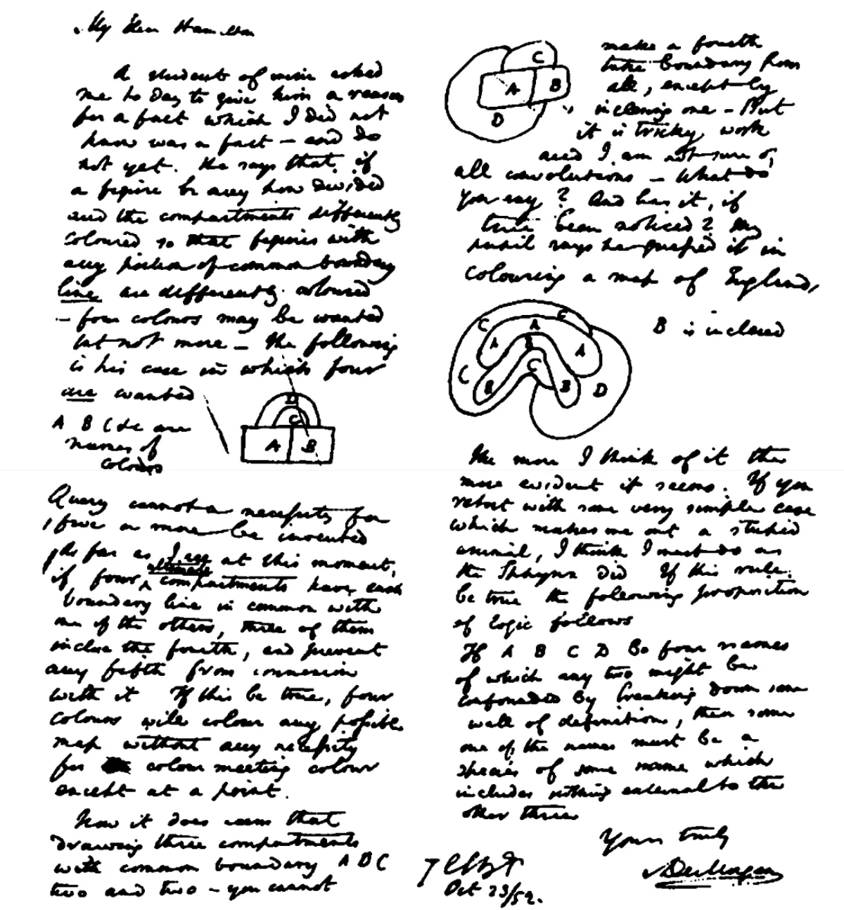
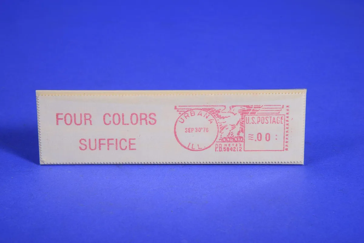
This is the colouring problem, and it is the mathematics of conflict-free assignment. The colours can be meeting hours, exam slots, radio frequencies, or the fast registers inside a processor. The rule is always the same: things that touch must differ. The most famous theorem of graph theory lives here. It says that the countries of any flat map can be coloured with four colours so that neighbouring countries always look different. That claim, made by a student in 1852, took 124 years to prove, and the proof needed a computer[1].
The chapter has a second, deeper story. When a graph needs many colours, can we always point to a concrete local reason, some dense cluster that forces the demand? The surprising answer is no: colour demand can be a purely global phenomenon, invisible under any local microscope. The final sections study the well-behaved graphs where that spookiness never happens.
Universities schedule final exams by exactly the committee trick: each exam is a vertex, an edge joins two exams that share a student, and the time slots are the colours. A survey by Qu, Burke, McCollum, Merlot and Lee reviews a decade of automated examination-timetabling systems; colouring-based construction methods are among the core techniques the field is built on[8]. Real timetables add soft wishes (spread exams out, respect room sizes), so colouring is the skeleton and heuristics add the flesh.
In the parliament example, when are two dots joined by a line?
New notation in this chapter
These are the symbols this chapter introduces. Skim the table now, then return to it whenever a symbol looks unfamiliar. Symbols from earlier chapters (\(V\), \(E\), \(\Delta\), \(K^n\), and friends) are re-explained where they appear.
| Symbol | Read it as | Meaning | Tiny example |
|---|---|---|---|
| \(c\colon V \to S\) | "a colouring c from V to S" | A rule assigning each vertex \(v\) a colour \(c(v)\) from a set \(S\), with adjacent vertices always coloured differently. | On a triangle \(abc\): \(c(a)=1\), \(c(b)=2\), \(c(c)=3\). |
| \(\chi(G)\) | "chi of G" | The chromatic number: the smallest number of colours that can properly colour the vertices of \(G\). | \(\chi(\text{triangle})=3\); \(\chi(\text{square})=2\). |
| \(\chi'(G)\) | "chi-prime of G" | The chromatic index: the smallest number of colours for the edges, where edges sharing an endpoint must differ. | \(\chi'(\text{triangle})=3\). |
| \(\mathrm{col}(G)\) | "the colouring number of G" | The least \(k\) such that the vertices can be listed in an order where each vertex has fewer than \(k\) neighbours earlier in the list. | Trees: \(\mathrm{col}=2\). |
| \((S_v)_{v \in V}\) | "the family of lists S-sub-v" | An assignment to each vertex \(v\) of its own personal menu \(S_v\) of permitted colours. | \(S_a=\{\text{red},\text{blue}\}\), \(S_b=\{\text{blue},\text{green}\}\). |
| \(\mathrm{ch}(G)\) | "the choice number of G" | The least \(k\) such that \(G\) can be coloured from the lists no matter which size-\(k\) menus are dealt. | \(\mathrm{ch}(K_{2,4})=3\) although \(\chi(K_{2,4})=2\). |
| \(\mathrm{ch}'(G)\) | "the list-chromatic index of G" | The edge version of the choice number: least \(k\) so that edges can always be coloured from any size-\(k\) menus. | Bipartite graphs: \(\mathrm{ch}'=\Delta\). |
| \(N^+(v)\), \(d^+(v)\) | "out-neighbourhood, out-degree of v" | In a directed graph: the set of vertices \(v\) points to, and how many there are. | In \(a \to b \to c \to a\): \(N^+(a)=\{b\}\), \(d^+(a)=1\). |
| \(\omega(G)\) | "omega of G" | The clique number: the size of the largest set of vertices that are all pairwise joined. | \(\omega(C^5)=2\): its biggest clique is a single edge. |
| \(\alpha(G)\) | "alpha of G" | The independence number: the size of the largest set of vertices with no edges among them. | \(\alpha(C^5)=2\). |
The table gives \(\omega(C^5) = 2\) for the five-cycle. Read correctly, this says:
Colouring vertices: the rules of the game
Here is the game stated once and carefully. Recall from Chapter 1 that a graph \(G\) has a vertex set \(V\) (the dots) and an edge set \(E\) (the lines), and that two vertices joined by an edge are called adjacent.
A vertex colouring of \(G\) is a map \(c\colon V \to S\) ("a rule \(c\) assigning to each vertex a colour from the set \(S\)") such that \(c(v) \ne c(w)\) whenever \(v\) and \(w\) are adjacent. The chromatic number \(\chi(G)\) is the smallest number \(k\) for which a colouring \(c\colon V \to \{1,\dots,k\}\) exists. In words: paint every dot so that dots joined by a line never share a paint; \(\chi(G)\) is the minimum paint budget.
Two small points of vocabulary carry a lot of weight later. \(G\) is \(k\)-colourable if \(k\) colours are enough, that is, \(\chi(G) \le k\). \(G\) is \(k\)-chromatic if \(\chi(G) = k\) exactly. "Colourable" is an upper-bound word; "chromatic" is an exact-value word. A square is 2-chromatic, and it is also 3-colourable, because more colours than you need is never a problem.
Why does the rule only restrict adjacent pairs? Because the applications only forbid conflicts between things that actually touch. Committees with no common member may happily meet at the same hour. The colours themselves have no identity; only their number matters, which is why we standardise to \(\{1, \dots, k\}\).
Look at what a colouring really does: it sorts the vertices into groups. The group of all vertices coloured \(i\) is called a colour class, and by the colouring rule no edge runs inside a class. A set of vertices with no edges among them is called an independent set, so a \(k\)-colouring is exactly a way of splitting the vertices into \(k\) independent sets. This reframing is worth memorising: it is what connects colouring to the independence number \(\alpha\) and to perfect graphs at the end of the chapter.
One family you already know settles the case of two colours. A graph is bipartite (from Chapter 1: its vertices split into two sides with all edges running between the sides) precisely when it is 2-colourable, and that happens precisely when it has no cycle of odd length. Odd cycles are the basic enemies of cheap colourings, and they will keep reappearing all chapter.
Edges can be coloured too, and the parallel theory turns out to behave completely differently.
An edge colouring of \(G\) is a map \(c\colon E \to S\) with \(c(e) \ne c(f)\) whenever the edges \(e\) and \(f\) share an endpoint. The chromatic index \(\chi'(G)\) ("chi-prime of G", also called the edge-chromatic number) is the least number of colours that suffices. In words: paint the lines so that lines meeting at a dot always differ.
All the edges at one vertex pairwise conflict, so a vertex with \(d\) edges forces \(d\) colours by itself. Writing \(\Delta(G)\) for the maximum degree (from Chapter 1: the largest number of edges touching any single vertex), we get \(\chi'(G) \ge \Delta(G)\) for free. The surprise of Section 5.3 below is how close to this floor every graph stays.
Edge colouring is secretly a special case of vertex colouring. Recall the line graph \(L(G)\): its vertices are the edges of \(G\), two of them adjacent when the original edges share an endpoint. Colouring the edges of \(G\) is literally the same task as colouring the vertices of \(L(G)\), so \(\chi'(G) = \chi(L(G))\)[1].
For edge colouring, two edges conflict when they share an endpoint. Whether two lines cross each other in your drawing is irrelevant; crossings are an accident of the picture, not a feature of the graph.
Colouring the vertices of \(G\) with \(k\) colours is the same thing as:
Why is \(\chi'(G) \ge \Delta(G)\) true for every graph, with no work at all?
Maps, and four colours for every planar graph
Colouring began with maps. Colour the countries of a map so that countries sharing a border stretch get different colours. Place a vertex in each country and join two vertices when their countries share a border: the result is a graph you can draw with no crossing edges, a planar graph in the sense of Chapter 4. Map colouring is vertex colouring of planar graphs.
Every planar graph \(G\) satisfies \(\chi(G) \le 4\): four colours suffice for the vertices of any graph drawable in the plane without crossings[1].
Four is best possible: the wheel of Figure 5.1 is planar and needs all four, and so does the complete graph \(K^4\) (four vertices, all pairs joined; many other books write \(K_4\) where Diestel writes \(K^4\)). The history is dramatic. Francis Guthrie posed the question in 1852 while colouring a map of England. Alfred Kempe published a proof in 1879; eleven years later Percy Heawood found a fatal error in it, and could salvage only a five-colour version. The full theorem waited until 1977, when Appel and Haken reduced it to 1,482 unavoidable configurations and had a computer verify, case by machine-checked case, that each one can be patched. No human-readable proof is known to this day, and the book states the theorem without proof[1]. What a human can do, in half a page, is one colour worse:
Every planar graph \(G\) satisfies \(\chi(G) \le 5\)[1].
The proof idea rewards a slow read, because its two tricks power half the chapter. Induct on the number of vertices. Planarity forces some vertex \(v\) with at most five neighbours (planar graphs have average degree below six, a consequence of Euler's formula from Chapter 4). Remove \(v\), colour the rest with five colours, and put \(v\) back. Trouble arises only if \(v\)'s five neighbours show all five colours. Now the first trick, the colour swap: look at just the vertices coloured 1 or 3. If \(v\)'s colour-1 neighbour and colour-3 neighbour lie in different connected pieces of that two-coloured subgraph, swap colours 1 and 3 throughout one piece. The swap keeps the colouring valid, and now colour 1 is free for \(v\). If instead the two neighbours are connected by a path alternating colours 1 and 3, that path plus \(v\) closes a ring, and planarity means the ring traps the colour-2 neighbour on one side and the colour-4 neighbour on the other. So the 2-versus-4 swap cannot be blocked, and it frees a colour for \(v\). (These alternating two-coloured pieces are classically called Kempe chains, salvaged from Kempe's failed proof.) The second trick appears in Diestel's alternative proof: contraction. Merge \(v\) with two of its non-adjacent neighbours into a single vertex, five-colour the smaller planar graph, and pull the colouring back; the two merged neighbours now share a colour, so \(v\) sees at most four colours and takes a fifth.
One more planar gem, stated without proof in the book: if a planar graph contains no triangle at all, three colours are enough (Grötzsch 1959)[1]. Forbidding a small substructure lowers the colour demand. Hold that thought; it becomes the main theme of the last two sections.
The Four Colour Theorem is about planar graphs only. General graphs need arbitrarily many colours: \(K^5\) needs five, \(K^{100}\) needs a hundred. And in map language the countries must be connected regions; an empire with two separated territories that must share one colour breaks the theorem.
Which statement follows from the Four Colour Theorem?
Greedy colouring, and the best possible degree bound
How would you actually colour a graph? The obvious algorithm is greedy: put the vertices in a row \(v_1, v_2, \dots, v_n\), then walk down the row and give each vertex the smallest colour number not already used on its earlier neighbours. Greedy always succeeds, and it never needs more than \(\Delta(G) + 1\) colours: when a vertex is coloured, its neighbours (at most \(\Delta\) of them) can block at most \(\Delta\) colours, so among \(\Delta + 1\) colours one is always free. That gives \(\chi(G) \le \Delta(G) + 1\) for every graph[2].
But greedy has a dark side: its output depends entirely on the ordering. Some ordering always achieves the true chromatic number (order a best colouring class by class and check), but a bad ordering can be catastrophic.
Run greedy on the crown graph of Figure 5.3 in the order \(a_1, b_1, a_2, b_2, a_3, b_3\). Vertex \(a_1\) takes colour 1. Vertex \(b_1\) is not adjacent to \(a_1\) (the crown omits the vertical pairs), so it also takes colour 1. Now \(a_2\) sees its neighbour \(b_1\) wearing 1, so it takes 2; \(b_2\) sees \(a_1\) wearing 1, so it takes 2. Then \(a_3\) sees \(b_1\) (colour 1) and \(b_2\) (colour 2) and must take 3, and \(b_3\) likewise. Three colours spent on a 2-chromatic graph, and the same pattern with \(n\) columns spends \(n\).
The lesson: greedy is only as good as its ordering. So the right question is, how well can greedy do under the best ordering? The answer has a name.
The colouring number \(\mathrm{col}(G)\) is the least \(k\) such that the vertices can be listed in an order in which every vertex is preceded by fewer than \(k\) of its own neighbours. Greedy along such an order uses at most \(k\) colours, so \(\chi(G) \le \mathrm{col}(G)\). In words: it measures the best "look-back degree" any ordering can achieve.
There is an exact formula, and it is beautifully concrete. Write \(\delta(H)\) for the minimum degree of a graph \(H\) (the smallest number of edges at any of its vertices). Then \[ \chi(G) \;\le\; \mathrm{col}(G) \;=\; \max\{\, \delta(H) : H \subseteq G \,\} + 1, \] read aloud: the colouring number equals one plus the largest minimum degree found in any subgraph \(H\) of \(G\)[2]. The ordering that achieves it is built backwards by peeling: pick a vertex of minimum degree in \(G\) and put it last; pick a minimum-degree vertex of what remains and put it second to last; repeat. Every vertex then looks back at few neighbours. For a tree this gives \(\mathrm{col} = 2\): peel leaves forever, and every vertex has only one earlier neighbour.
A first consequence: dense cores are unavoidable. Diestel proves that every graph needing \(k\) colours contains a subgraph that still needs \(k\) colours and in which every vertex has at least \(k-1\) neighbours (Lemma 5.2.3)[2]. The reason: take a smallest piece still needing \(k\) colours. If some vertex \(v\) of it had at most \(k-2\) neighbours, colour the rest with \(k-1\) colours (possible, by smallestness) and note that \(v\)'s few neighbours cannot block all \(k-1\) colours. There is also a bound from the edge count alone: an optimal colouring must have at least one edge between every pair of colour classes (otherwise merge the two classes into one colour), so \(k\) classes force at least \(\tfrac{1}{2}k(k-1)\) edges. Many colours require many edges[2].
Can the greedy bound \(\Delta + 1\) itself be improved? Almost always, and the exceptions can be listed exactly. Two families genuinely need \(\Delta + 1\) colours: the complete graph \(K^n\) (every vertex has degree \(n-1\), and all \(n\) vertices need distinct colours) and the odd cycles (degree 2 everywhere, chromatic number 3). Brooks proved in 1941 that these are the only culprits.
Let \(G\) be a connected graph that is neither complete nor an odd cycle. Then \(\chi(G) \le \Delta(G)\)[2].
The proof idea: suppose some connected, non-complete, non-odd-cycle \(G\) needed \(\Delta + 1\) colours. Remove a vertex \(v\), colour the rest with \(\Delta\) colours, and study why the colouring cannot be extended: \(v\)'s neighbours must show all \(\Delta\) colours, and any two of them must be joined by a path alternating between their two colours (otherwise a Kempe-chain swap, as in the Five Colour Theorem, frees a colour). A careful analysis of how these alternating paths can and cannot intersect either finds a recolouring that frees a colour, or forces every pair of \(v\)'s neighbours to be adjacent, which makes \(G\) complete. The full case analysis is in Diestel §5.2 and is a workout, not a stroll.
Greedy does not compute \(\chi(G)\). It computes an upper bound whose quality depends on the vertex order: at worst \(\Delta(G)+1\), at best \(\chi(G)\), with the peeling order guaranteeing \(\mathrm{col}(G)\). And Brooks's theorem does not say \(\chi \le \Delta\) for every graph: complete graphs and odd cycles genuinely need \(\Delta + 1\), and the statement assumes \(G\) is connected (otherwise apply it to each piece).
When a compiler translates your program, it must decide which variables live in the processor's few fast registers. Gregory Chaitin's classic method at IBM builds an interference graph: one vertex per variable, an edge whenever two variables are alive at the same moment and so cannot share a register. Allocating \(k\) registers is then colouring this graph with \(k\) colours; when the graph resists, a variable is "spilled" to slower memory[7]. Chaitin's retrospective records that the technique was built for IBM's 801 project, ancestor of the RS/6000 and PowerPC processors, and that the designers moved from 16 to 32 registers partly because the colouring allocator used extra colours so effectively[7]. A colouring theorem helped size a real processor family.
Greedy colours the crown graph of Figure 5.3 with three colours although \(\chi = 2\). What does this show?
\(G\) is connected with \(\Delta(G) = 3\). Which extra fact lets you conclude \(\chi(G) \le 3\)?
When high colour demand has no local cause
Every bound so far ties colours to something you can see: degrees, edges, dense cores. Here is the natural next question. If a graph needs \(k\) colours, must it contain a concrete witness, say a cluster of \(k\) mutually joined vertices? A clique of size \(k\) certainly forces \(k\) colours all by itself. Is it the only way?
Erdős answered this in 1959, and the answer reshaped the subject. Recall the girth \(g(G)\) from Chapter 1: the length of the shortest cycle in \(G\). Large girth means no short cycles at all, so around any vertex the graph looks like a tree, and trees are 2-colourable.
For every integer \(k\) there exists a graph \(G\) with girth \(g(G) > k\) and chromatic number \(\chi(G) > k\)[2].
Read that twice. There are graphs that need more than a thousand colours, yet contain no cycle shorter than a thousand: no triangle, no square, nothing small. Zoom in anywhere and you see a tree, locally colourable with 2 colours. The demand for a thousand colours is real, but it is a property of the whole, not of any part. No picture of such a graph can be drawn at page scale, and that is precisely the point. Even the proof refuses to point at an example: it is probabilistic (given in Chapter 11), showing that a suitable random graph has, with positive probability, few short cycles and no large independent set. Few short cycles can be repaired by deleting a vertex from each; no large independent set forces many colours, because colour classes are independent sets. Counting shows such graphs must exist without exhibiting one; explicit constructions came later, and are much harder.
Think of colour demand as a property like the temperature of a gas rather than the shape of a molecule. Erdős's theorem says you can have heat with no single hot spot: every local reading looks cool (tree-like, 2-colourable), yet globally the graph is scorching. Any theory that explains chromatic number by pointing at small pieces is doomed from the start.
Doomed, unless you change what counts as a witness. Hajós proposed certificates that are not small pieces but constructions. Call a graph \(k\)-constructible if it can be built by three rules: start from the complete graph \(K^k\); or take a constructed graph with two non-adjacent vertices \(x, y\), add the edge \(xy\), and contract it to a single vertex; or take two constructed graphs sharing exactly one vertex \(x\), with an edge \(x y_1\) in the first and \(x y_2\) in the second, delete both those edges and add the edge \(y_1 y_2\) instead. Each rule provably preserves the property "needs at least \(k\) colours".
\(\chi(G) \ge k\) if and only if \(G\) contains a \(k\)-constructible subgraph[2].
Figure 5.5 shows the machine certifying that the five-cycle needs three colours. Why does the rule preserve the demand? Suppose the right-hand graph had a proper 2-colouring \(c\). If \(c(x) \ne c(y_1)\), then \(c\) would still be proper after restoring the edge \(x y_1\), making the left triangle 2-colourable: impossible. So \(c(x) = c(y_1)\), and by the same argument \(c(x) = c(y_2)\). But then \(y_1\) and \(y_2\) share a colour while joined by the new edge. Contradiction, with no colouring ever attempted. A caution from Diestel's notes: this is a complete generative grammar for colour demand, but not a usable certificate in the algorithmic sense, since no bound is known on how long a construction must be. Compare Kuratowski's theorem in Chapter 4, where the witness for non-planarity is one small, findable subgraph; nothing like that can exist for \(\chi \ge k\), by Erdős's theorem, since any witness containing a cycle is absent from graphs of large girth.
"A graph needs many colours only if it has a big clique." False, and it is the chapter's central surprise. Erdős's theorem gives triangle-free graphs (clique number 2) with chromatic number beyond any bound. Big cliques force many colours; many colours do not force big cliques.
Erdős's theorem supplies a graph with girth above 1000 and \(\chi\) above 1000. How big is its largest clique?
Colouring edges: the tame world of König and Vizing
Now colour the edges instead, so that edges meeting at a vertex differ. We saw that \(\chi'(G) \ge \Delta(G)\) always: the busiest vertex is an obvious bottleneck. For bipartite graphs, the obvious bottleneck is the only one.
Every bipartite graph \(G\) satisfies \(\chi'(G) = \Delta(G)\)[3].
Proof idea: induct on the number of edges. Remove an edge \(xy\), colour the rest with \(\Delta\) colours, and put \(xy\) back. Some colour \(\alpha\) is unused at \(x\) and some colour \(\beta\) unused at \(y\) (each vertex has at most \(\Delta\) edges). If \(\alpha = \beta\), use it on \(xy\). Otherwise, follow the path starting at \(x\) whose edges alternate \(\beta, \alpha, \beta, \alpha, \dots\). In a bipartite graph this path can never come back around to \(y\): doing so would close a cycle of odd length, and bipartite graphs have none. So swap \(\alpha\) and \(\beta\) along the path; now \(\beta\) is free at both \(x\) and \(y\), and colours \(xy\).
König's theorem solves the school timetable problem exactly. Teachers on one side, classes on the other, one edge per required lesson: the graph is bipartite, and the number of periods needed equals \(\Delta\), the load of the busiest teacher or class. No cleverness beyond that busiest load is ever required. And for general, non-bipartite graphs? Here is the theorem this chapter calls astonishing.
Every graph \(G\) satisfies \(\Delta(G) \;\le\; \chi'(G) \;\le\; \Delta(G) + 1\)[3].
Whatever graph you hand me, its chromatic index is one of exactly two consecutive values. Compare the chromatic number, which can sit anywhere from 2 up to \(\Delta + 1\) and, by Erdős, resists all local explanation. Graphs with \(\chi' = \Delta\) are called class 1; graphs with \(\chi' = \Delta + 1\) are class 2. Even cycles are class 1; odd cycles are class 2 (two edge-colours cannot get around an odd ring, exactly as in Figure 5.2). The proof of Vizing's theorem runs an induction on edges with \(\Delta + 1\) colours as the target. At every vertex at least one colour is missing (there are \(\Delta+1\) colours but at most \(\Delta\) edges). The argument builds a "fan" of edges around a stuck vertex, rotates colours around the fan, and follows paths that alternate between two colours, swapping them along the way; the details are in Diestel §5.3 and use nothing beyond patience.
Two remarks complete the picture. First, being class 2 costs exactly one extra colour, never more; the hard part is telling the classes apart, for which no efficient certificate is known. Second, a landmark from 2016: Csaba, Kühn, Lo, Osthus and Treglown proved that all sufficiently large \(d\)-regular graphs on an even number \(n\) of vertices with \(d \ge n/2\) are class 1[3]. Dense regular graphs of even order always decompose into perfect one-round schedules; class-2 behaviour is a phenomenon of sparse or irregular graphs. (Even order is needed: with \(n\) odd, no round can cover everyone.)
The five-cycle \(C^5\) has \(\Delta = 2\). What is its chromatic index \(\chi'(C^5)\)?
List colouring: when every vertex brings its own menu
Now a twist that sounds like a technicality and turns out to be a different world. Suppose each vertex \(v\) is handed its own personal list \(S_v\) of allowed colours, and we must find a proper colouring \(c\) with \(c(v) \in S_v\) for every \(v\): each vertex's colour drawn from its own menu. When can we always succeed?
\(G\) is \(k\)-choosable if for every family of lists \((S_v)_{v \in V}\) with all \(|S_v| = k\), a proper colouring from the lists exists. The choice number \(\mathrm{ch}(G)\) is the least such \(k\). The edge version: \(\mathrm{ch}'(G) := \mathrm{ch}(L(G))\), the least \(k\) such that the edges can always be coloured from any size-\(k\) lists[4].
The quantifier is the whole point: an adversary deals the menus, and you must win against every deal. One possible deal is "everyone gets \(\{1, \dots, k\}\)", which is ordinary \(k\)-colouring. So \(k\)-choosable implies \(k\)-colourable, and \(\mathrm{ch}(G) \ge \chi(G)\) always. Intuition says varied menus should make life easier, since neighbours with disjoint menus cannot even conflict. The intuition is backwards, and here is the smallest counterexample.
In Figure 5.7 the graph is bipartite, so \(\chi = 2\). But against the lists shown, \(u_1\) picks from \(\{1,2\}\) and \(u_2\) from \(\{3,4\}\), and the four possible pairs \((1,3), (1,4), (2,3), (2,4)\) are exactly the four lists on the right side. Whichever pair is chosen, one \(w_j\) finds both of its options already on its neighbours. So \(\mathrm{ch}(K_{2,4}) \ge 3\): menus genuinely cost more. And the gap is not a small-example artefact. Alon proved in 1993 that sheer average degree forces the choice number up: there is a function \(f\) such that every graph of average degree at least \(f(k)\) has \(\mathrm{ch}(G) \ge k\)[4]. Contrast \(\chi\): the complete bipartite graphs \(K_{n,n}\) are as dense as you like and still 2-chromatic. Choosability and colourability are fundamentally different invariants. The reason colour-density tricks fail here: swapping two colours along a Kempe chain assumes the two colours are available everywhere along the chain, and private menus break that assumption.
Given all this, the next theorem is remarkable. Thomassen proved in 1994 that every planar graph is 5-choosable[4]. The proof is a famous jewel: barely a page, no computer, and it does not even use Euler's formula. The trick is to prove something stronger so that induction has room to move: for a plane graph whose outer boundary is a cycle, with two adjacent boundary vertices pre-coloured, all other boundary vertices holding lists of size 3, and all interior vertices holding lists of size 5, the colouring always extends. Cutting along a chord, or peeling one boundary vertex while reserving two of its list colours, makes the induction close on itself. Since 5-choosable implies 5-colourable, this re-proves the Five Colour Theorem in passing. It is also best possible: Voigt constructed a planar graph that is not 4-choosable, so the Four Colour Theorem does not survive the upgrade to lists[4].
"Bigger variety in the menus should make list colouring easier." Backwards: \(k\)-choosability must beat every deal, including the all-identical deal, so it is the harder property and \(\mathrm{ch}(G) \ge \chi(G)\). Also tempting and false: "planar graphs are 4-choosable since they are 4-colourable." Thomassen's 5 is sharp.
For edge colouring, though, menus are conjectured to cost nothing at all. The List Colouring Conjecture states that \(\mathrm{ch}'(G) = \chi'(G)\) for every graph; it is open, and it is the central open problem of the area[4]. The bipartite case was proved by Galvin in 1995, and the proof runs on machinery from a different chapter entirely: stable matchings.
The bridge is the notion of a kernel. Orient the graph: give each edge a direction, making a directed graph \(D\). Write \(N^+(v)\) for the out-neighbourhood of \(v\) (the set of vertices \(v\) points to) and \(d^+(v)\) for the out-degree (how many there are). A kernel of \(D\) is an independent set \(U\) such that every vertex outside \(U\) sends at least one directed edge into \(U\). Think of a committee with no internal conflicts, such that every outsider defers to at least one member.
Kernels are fragile: the directed triangle in Figure 5.8 has none, and directed odd cycles are the basic obstruction. But when they do exist, they deliver list colourings. Diestel's kernel lemma (Lemma 5.4.3) says: if a graph has an orientation in which every vertex's out-degree is smaller than its list size, and every induced subgraph of the orientation has a kernel, then the graph can be coloured from the lists[4]. The proof colours one colour at a time: pick a colour \(\alpha\), look at the vertices whose lists contain it, take a kernel \(U\) of that region, give everyone in \(U\) the colour \(\alpha\) (legal, since kernels are independent), and delete \(\alpha\) from the other lists in the region. Each such vertex points into \(U\), so its out-degree drops at least as fast as its list shrinks, and the induction survives.
Every bipartite graph \(G\) satisfies \(\mathrm{ch}'(G) = \chi'(G)\): for bipartite graphs, list edge colouring costs no more than ordinary edge colouring[4].
The proof orients the line graph of \(G\) using a fixed optimal edge colouring as a ranking, so that each edge points at fewer than \(\chi'(G)\) others. The kernels demanded by the kernel lemma are then supplied by the stable marriage theorem from Chapter 2: read the orientation as preference rankings at each vertex, and a stable matching is exactly a kernel. A theorem about stable preferences proves a theorem about colouring. Combining Galvin with König gives a clean corollary: every bipartite graph satisfies \(\mathrm{ch}'(G) = \Delta(G)\). The school timetable survives personal menus: even if every lesson comes with its own set of allowed periods, as long as each menu has \(\Delta\) entries, the timetable can be filled.
The stable matching engine inside Galvin's proof is itself deployed infrastructure. Gale and Shapley's 1962 paper posed the college admissions problem and gave the deferred acceptance procedure that always finds a stable assignment[10]. The National Resident Matching Program, which assigns graduating medical students in the United States to hospital residency programs, runs an applicant-proposing version of exactly this mechanism: tentative matches can be bumped as better-ranked applicants arrive, and the process settles into a stable final match[11]. One algorithmic idea, two lives: matching doctors to hospitals, and certifying kernels for list colourings.
Radio and cellular networks assign frequencies so that nearby transmitters do not interfere: transmitters are vertices, potential interference is an edge, frequencies are colours. The survey by Aardal, van Hoesel, Koster, Mannino and Sassano organizes the field's models, which are built on generalizations of graph colouring in which edges carry separation requirements rather than a bare "must differ"[9]. And when each transmitter is licensed for only some bands, its allowed set is precisely a list in the sense of this section: list colouring is the natural model for restricted availability.
With the lists of Figure 5.7 the graph \(K_{2,4}\) cannot be coloured, yet \(\chi(K_{2,4}) = 2\). What follows?
Why does the directed triangle \(x \to y \to z \to x\) have no kernel?
Perfect graphs: when colour demand always has a local explanation
Erdős's theorem showed that in general, chromatic number can float free of all local structure. The last two sections ask: in which graphs does that never happen? Two quantities frame the question. The clique number \(\omega(G)\) ("omega of G") is the size of the largest complete subgraph: the biggest cluster of pairwise-joined vertices. The independence number \(\alpha(G)\) ("alpha of G") is the size of the largest independent set: the biggest conflict-free crowd. The two are mirror images: recall the complement \(\overline{G}\) (same vertices, with exactly the missing edges); then \(\alpha(G) = \omega(\overline{G})\). Cliques bound colouring from below, \(\chi(G) \ge \omega(G)\), since a clique of size \(r\) needs \(r\) colours by itself. Independence bounds it from the other side: each colour class is an independent set of size at most \(\alpha(G)\), so \(\chi(G) \ge |G| / \alpha(G)\), where \(|G|\) is the number of vertices.
\(G\) is perfect if every induced subgraph \(H\) of \(G\) satisfies \(\chi(H) = \omega(H)\). (Induced subgraph, from Chapter 1: pick a set of vertices and keep all the edges of \(G\) between them.) In words: at every zoom level, the paint budget is exactly explained by the biggest cluster.
Why quantify over all induced subgraphs rather than just ask \(\chi(G) = \omega(G)\)? Because a single lucky coincidence means nothing. Take a five-cycle plus a separate triangle: the whole graph has \(\chi = 3 = \omega\), yet the five-cycle hiding inside needs three colours with no triangle to blame. Requiring the equation at every zoom level makes perfection a genuine structural property rather than an accident. Bipartite graphs are perfect (every induced piece with an edge has \(\chi = 2 = \omega\)). The five-cycle is the smallest imperfect graph: \(\omega(C^5) = 2\) but \(\chi(C^5) = 3\).
A rich family of perfect graphs comes from forbidding hollow rings. Call a cycle of length at least 4 in \(G\) induced when it has no chord, no edge of \(G\) joining two of its non-consecutive vertices. A graph is chordal if it has no induced cycle of length 4 or more: every big ring is braced by a chord.
Diestel proves two structural facts. First (Proposition 5.5.1): the chordal graphs are exactly the graphs you can build recursively by pasting complete graphs together along complete overlaps, as in Figure 5.9. (Pasting: \(G\) is the union of induced subgraphs \(G_1\) and \(G_2\) whose intersection is \(S\); we say \(G\) is pasted from them along \(S\).) The key step: in a chordal graph, any minimal set of vertices separating two others must be complete, or a shortest path around each side would close an unbraced ring. Second (Proposition 5.5.2): every chordal graph is perfect. The reason pasting preserves perfection is a pleasant colour argument: colour each half optimally with \(\omega\) colours; on the complete overlap, each colouring uses all distinct colours, so the two colourings can be rotated to agree there and merged[5]. Interval graphs, which model overlapping time intervals and appear in scheduling and genetics, are chordal, so optimal colouring is tractable for them; the interference graphs of straight-line program code are of this kind, one reason the register allocation story of Section 5.2 works so well in practice.
Which graphs are perfect in general? Berge conjectured the answer in 1963, in terms of two forbidden shapes. A hole of \(G\) is an induced cycle of length at least 4; an antihole is a hole of the complement \(\overline{G}\). An odd hole (length at least 5) is imperfect on its own, as \(C^5\) shows, and so is an odd antihole. Berge's conjecture, that these are the only obstructions, was proved forty years later in a 179-page argument.
A graph is perfect if and only if neither it nor its complement contains an odd cycle of length at least 5 as an induced subgraph: perfect = no odd holes and no odd antiholes[5].
The theorem's proof follows the same architecture as the chordal case, scaled up enormously: decompose every graph without odd holes and antiholes into basic perfect pieces along perfection-preserving joins. The book, honestly, declines to sketch further, and so do we; the point to keep is that a quantified statement over all induced subgraphs became a concrete forbidden-shape test, and perfection is even decidable in polynomial time. Long before the strong theorem, Lovász proved Berge's easier conjecture, with a proof you can hold in your head.
A graph is perfect if and only if its complement is perfect[5].
Cliques of \(G\) are independent sets of \(\overline{G}\) and vice versa, so the theorem says perfection is symmetric between the two viewpoints. The proof pivots on replication: from \(G\) and a vertex \(x\), build \(G'\) by adding a clone \(x'\) joined to \(x\) and to all of \(x\)'s neighbours. The Replication Lemma says cloning preserves perfection, and repeated cloning lets one make overlapping maximum independent sets disjoint, extract a clique meeting all of them, and convert colourings of \(G\) into clique covers of \(\overline{G}\). Lovász also proved a purely numerical characterization: \(G\) is perfect exactly when every induced subgraph \(H\) satisfies \(|H| \le \alpha(H) \cdot \omega(H)\), vertex count at most crowd size times clique size[5]. The five-cycle fails it: \(5 > 2 \times 2\). Since \(\alpha\) and \(\omega\) trade places under complementation, this inequality is complement-symmetric on its face, and the Perfect Graph Theorem drops out instantly. Gasparian's proof of the hard direction is a half-page of linear algebra, building incidence matrices whose product is invertible and comparing ranks; it is one of the most admired short proofs in combinatorics, and it lives in Diestel §5.5.
Perfection is not "\(\chi = \omega\) for this graph"; it demands the equation for every induced subgraph. And a hole is not any cycle: it is an induced cycle of length at least 4, chords disqualify it. Only odd holes and odd antiholes obstruct perfection; even holes are harmless, as every bipartite graph full of 4-cycles shows.
\(G\) is a five-cycle together with a separate triangle, so \(\chi(G) = \omega(G) = 3\). Is \(G\) perfect?
Relaxing perfection: chi-bounded classes
Perfect graphs demand the exact equation \(\chi = \omega\) everywhere. A looser, more forgiving question: in which classes of graphs is \(\chi\) at least controlled by \(\omega\), so that small cliques imply not-too-many colours? A class of graphs closed under induced subgraphs is called \(\chi\)-bounded ("chi-bounded") if there is some function \(f\) with \(\chi(G) \le f(r)\) for every member \(G\) whose clique number is at most \(r\)[6]. Perfect graphs are the extreme case \(f(r) = r\). Any \(f\) will do; the question is only whether colour demand can run away from clique size inside the class.
Erdős's theorem says the class of all graphs is not \(\chi\)-bounded, and neither is the class of triangle-free graphs: girth-and-chromatic-number graphs are triangle-free with unbounded \(\chi\). So which forbidden shapes tame a class? Two highlights close the chapter. Scott and Seymour proved in 2016 that the graphs with no odd hole form a \(\chi\)-bounded class: half of the Strong Perfect Graph Theorem's hypothesis, antiholes fully allowed, still buys the qualitative conclusion[6]. And Gyárfás proved that for any fixed path \(P\), the graphs not containing \(P\) as an induced subgraph form a \(\chi\)-bounded class. The proof is a double induction worth seeing in the book: grow a path from a well-chosen vertex, observe that each leftover component attaches to the path's neighbourhood, and recurse with a shorter forbidden path inside neighbourhoods of smaller clique number[6].
The guiding open problem of the area is the Gyárfás–Sumner conjecture: for any fixed forest \(F\) (any graph with no cycles at all), the graphs not containing \(F\) as an induced subgraph should be \(\chi\)-bounded. Forests are the only possible candidates: any forbidden shape containing a cycle is dodged by Erdős's large-girth graphs, which have \(\omega = 2\) and huge \(\chi\). The conjecture says every forest works; paths are the proved case. Between perfection's exact equation and Erdős's total anarchy runs a whole research frontier, and it is open in both directions.
Where next? Colouring feeds forward across the course: Chapter 6 turns map colouring into a statement about flows through networks, its geometric dual; Chapter 9 uses Brooks-style and Erdős-style bounds in Ramsey theory; Chapter 11 finally proves Erdős's theorem with random graphs; and Chapter 12 reuses the chordal decomposition as the seed of tree-decompositions and graph minors.
Why does the Gyárfás–Sumner conjecture forbid only forests, never a shape containing a cycle?
Check your understanding
What does \(\chi(G)\) stand for?
"\(G\) is 3-colourable" means:
The chromatic index \(\chi'(G)\) is the least number of colours needed so that:
Brooks's theorem says \(\chi(G) \le \Delta(G)\) for every connected graph except which two kinds?
A graph has maximum degree \(\Delta(G) = 6\). By Vizing's theorem, its chromatic index \(\chi'(G)\) must be:
A bipartite graph in which the busiest vertex has 5 edges is to be edge-coloured with as few colours as possible. How many are needed?
Which statement about the greedy colouring algorithm is correct?
The 5-cycle \(C^5\) has clique number \(\omega = 2\) and chromatic number \(\chi = 3\). What does this show?
Erdős proved that for every \(k\) there is a graph with no cycle shorter than \(k\) and chromatic number above \(k\). Which conclusion follows?
Every vertex of \(G\) is handed its own list of \(k\) allowed colours, and \(G\) can always be coloured from the lists, whatever size-\(k\) lists are dealt (\(G\) is \(k\)-choosable). Which statement must be true?
Sources and further reading
- R. Diestel, Graph Theory, 6th ed., Springer GTM 173 (2024), Chapter 5 introduction and §5.1 (Four Colour Theorem 5.1.1, Five Colour Theorem 5.1.2, Grötzsch's theorem 5.1.3; history in the chapter notes).
- R. Diestel, Graph Theory, 6th ed., Springer GTM 173 (2024), §5.2 (greedy bound, colouring number 5.2.2, Lemma 5.2.3, Brooks's theorem 5.2.4, Erdős's theorem 5.2.5, Hajós's theorem 5.2.6).
- R. Diestel, Graph Theory, 6th ed., Springer GTM 173 (2024), §5.3 (König's theorem 5.3.1, Vizing's theorem 5.3.2, Csaba–Kühn–Lo–Osthus–Treglown theorem 5.3.3).
- R. Diestel, Graph Theory, 6th ed., Springer GTM 173 (2024), §5.4 (Alon's theorem 5.4.1, Thomassen's theorem 5.4.2, kernel lemma 5.4.3, Galvin's theorem 5.4.4 and Corollary 5.4.5; List Colouring Conjecture and Voigt's example, with notes).
- R. Diestel, Graph Theory, 6th ed., Springer GTM 173 (2024), §5.5 (chordal structure 5.5.1–5.5.2, Strong Perfect Graph Theorem 5.5.3, Perfect Graph Theorem 5.5.4, Replication Lemma 5.5.5, Lovász's product characterization 5.5.6).
- R. Diestel, Graph Theory, 6th ed., Springer GTM 173 (2024), §5.6 (Scott–Seymour theorem 5.6.1, Gyárfás's proposition 5.6.2, Gyárfás–Sumner conjecture).
- G. J. Chaitin, "Register Allocation and Spilling via Graph Coloring", SIGPLAN Symposium on Compiler Construction (1982); reprinted with a retrospective in Best of PLDI 1979–1999, ACM SIGPLAN (2003). Full PDF.
- R. Qu, E. K. Burke, B. McCollum, L. T. G. Merlot, S. Y. Lee, "A survey of search methodologies and automated system development for examination timetabling", Journal of Scheduling 12 (2009), 55–89. Publisher page.
- K. I. Aardal, S. P. M. van Hoesel, A. M. C. A. Koster, C. Mannino, A. Sassano, "Models and solution techniques for frequency assignment problems", Annals of Operations Research 153 (2007), 79–129. Publisher page.
- D. Gale, L. S. Shapley, "College Admissions and the Stability of Marriage", The American Mathematical Monthly 69 (1962), 9–15. Full PDF.
- National Resident Matching Program, "How the Matching Algorithm Works", official explainer (accessed 2026). nrmp.org.