Part II · The Classic Theory
Chapter 6: Flows
Water in pipes, current in wires, freight on rails: this chapter turns "how much can move through this network?" into a theorem, and then discovers that colouring a map is the same question seen from the other side.
From pipes to bottlenecks
Picture a graph as a system of pipes. Each vertex is a junction. Each edge is a pipe, and something moves along it: water, electric current, data, trains. The mathematics of this picture keeps exactly one law from physics. At an ordinary junction, whatever comes in must go out. Nothing pools at a vertex, and nothing appears from nowhere. Electrical engineers call this conservation rule Kirchhoff's law, and it will sit at the centre of every definition in this chapter.
Two different questions grow out of the picture, and the chapter answers both. The first is practical. Suppose one special vertex, the source, pumps material into the system, another special vertex, the sink, drains it out, and every pipe has a stamped maximum capacity. How much can we ship from source to sink? The answer is the max-flow min-cut theorem of Ford and Fulkerson: the most you can push through equals the capacity of the tightest bottleneck separating the source from the sink. That single sentence powers a large share of applied graph theory, from routing freight to cutting objects out of photographs.
The second question is structural, and stranger. Forget capacities and forget the source and sink. Ask instead: can the graph carry a perfectly balanced flow that actually uses every edge, with no pipe left idle? Here the chapter makes an unexpected move. It measures flow not with ordinary numbers but with clock arithmetic, where values wrap around like hours on a clock face. Out of this comes the flow number of a graph, a quantity that behaves like a mirror image of the chromatic number \(\chi\) from Chapter 5 (the least number of colours a graph's vertices need). The mirror is literal: for a graph drawn in the plane, its chromatic number equals the flow number of its planar dual. Map colouring, including the four colour theorem, turns out to be the planar shadow of flow theory. And the chapter ends at an open frontier: three conjectures of Tutte, unproved since the 1950s, 60s and 70s, with Seymour's six-flow theorem as the best general result known.[6]
One housekeeping note. Throughout this chapter, graphs are allowed to be multigraphs: two vertices may be joined by several parallel edges, and an edge may loop from a vertex back to itself. Flows genuinely need this generality (duals of plane graphs often have parallel edges). Everything we prove holds for multigraphs, and we will say "graph" without fuss.
This chapter grows two questions out of the pipe picture. What makes the second one different from the first?
New notation in this chapter
Flow theory runs on careful bookkeeping about direction. The graph itself stays undirected; it is the flow that has a direction on each edge. The notation below exists to keep those directions straight, and every later section uses it. Skim the table now, then return to it whenever a symbol looks unfamiliar.
| Symbol | Read it as | Meaning | Tiny example |
|---|---|---|---|
| \((e,x,y)\) | "edge \(e\), travelled from \(x\) to \(y\)" | An oriented edge: the edge \(e=xy\) bundled with one of its two travel directions. A non-loop edge has two orientations; a loop has one. | If \(e\) joins \(a\) and \(b\), its orientations are \((e,a,b)\) and \((e,b,a)\). |
| \(\vec{e}\), \(\overleftarrow{e}\) | "\(e\) one way; \(e\) the reverse way" | Names for the two orientations of an edge \(e\); \(\overleftarrow{e}\) is whichever direction \(\vec{e}\) is not. | If \(\vec{e}=(e,a,b)\) then \(\overleftarrow{e}=(e,b,a)\). |
| \(\vec{E}\) | "the oriented edges of \(G\)" | Every edge of \(G\) listed once per direction. | A graph with 3 edges and no loops has 6 oriented edges. |
| \(\overline{X}\) | "\(X\) bar" | The complement of a vertex set: \(\overline{X}=V\setminus X\), all vertices not in \(X\). | If \(V=\{a,b,c,d\}\) and \(X=\{a,b\}\), then \(\overline{X}=\{c,d\}\). |
| \(\vec{F}(X,Y)\) | "the oriented edges in \(\vec{F}\) from \(X\) to \(Y\)" | The members of a set \(\vec{F}\) of oriented edges that start in \(X\) and end in \(Y\). Loops never count. | \(\vec{E}(x,V)\), also written \(\vec{E}(x)\): every direction leaving the vertex \(x\). |
| \(f(X,Y)\) | "the total flow from \(X\) to \(Y\)" | The sum of \(f\) over all oriented edges from \(X\) to \(Y\). | \(f(v,V)\) is the net amount leaving vertex \(v\). |
| (F1) | "antisymmetry" | \(f(e,x,y)=-f(e,y,x)\): reversing your point of view flips the sign. | "3 units from \(a\) to \(b\)" equals "\(-3\) units from \(b\) to \(a\)". |
| (F2) | "Kirchhoff's law" | \(f(v,V)=0\) at every vertex: in equals out everywhere. | One unit in, one unit out: balanced. |
| \(N=(G,s,t,c)\) | "a network" | A multigraph \(G\) with a source \(s\), a sink \(t\), and a capacity \(c(\vec{e})\) for each oriented edge. | Figure 6.3 shows a network on four vertices. |
| (F2′), (F3) | "balance except at \(s,t\); capacity limit" | (F2′): \(f(v,V)=0\) for every \(v\) other than \(s\) and \(t\). (F3): \(f(\vec{e})\le c(\vec{e})\) on every oriented edge. | A flow of 5 through a pipe of capacity 3 violates (F3). |
| \(|f|\) | "the total value of \(f\)" | The net flow across any source-side/sink-side frontier; the same number for every frontier, and equal to \(f(s,V)\). | The flow of Figure 6.3 has \(|f|=4\). |
| \(H\) | "the value group" | The number system flow values live in: any set with an addition that is commutative, has a zero, and has negatives (an "abelian group"). | The integers \(\mathbb{Z}\); the clock arithmetics \(\mathbb{Z}_k\). |
| \(\mathbb{Z}_k\) | "the integers modulo \(k\)" | Clock arithmetic with \(k\) positions \(0,1,\dots,k-1\); sums wrap around. | In \(\mathbb{Z}_3\): \(2+2=1\). |
| \(\mathbb{Z}_m\times\mathbb{Z}_n\) | "\(\mathbb{Z}_m\) cross \(\mathbb{Z}_n\)" | Pairs \((a,b)\), added coordinate by coordinate. It has \(m\cdot n\) elements. | In \(\mathbb{Z}_2\times\mathbb{Z}_3\): \((1,2)+(1,2)=(0,1)\). |
| \(\varphi(G)\) | "the flow number of \(G\)" | The least \(k\) such that \(G\) has a k-flow; \(\infty\) if there is none. | \(\varphi(K^4)=4\). |
| \(\sigma_k\) | "sigma \(k\)" | The remainder map from \(\mathbb{Z}\) to \(\mathbb{Z}_k\): each integer goes to its remainder modulo \(k\). | \(\sigma_3(5)=\bar{2}\). |
| \(\vec{C}\), \(\vec{P}\) | "\(C\) (or \(P\)) with an orientation" | A cycle, or a path, with a chosen direction of travel, recorded edge by edge. | The triangle \(abc\) travelled \(a\to b\to c\to a\). |
| \(F^*\), \(\vec{e}^{\,*}\) | "\(F\) star; \(e\) star" | For a plane graph and its dual: the dual edges of the edges in \(F\); and the oriented dual edge of \(\vec{e}\), obtained by rotating \(\vec{e}\) clockwise onto its dual edge. | Each side of a square corresponds to the dual edge crossing it. |
The table lists (F1) as \(f(e,x,y)=-f(e,y,x)\). Read correctly, what does that line say?
Circulations: balance everywhere
Our graphs are undirected, but flow has a direction. The trick that reconciles the two is to treat "edge plus direction" as an object in its own right. An oriented edge is a triple \((e,x,y)\), read "edge \(e\), travelled from \(x\) to \(y\)". Every edge \(e=xy\) that is not a loop gives rise to exactly two oriented edges, \((e,x,y)\) and \((e,y,x)\), one for each way of driving down it. Why a triple and not just the pair \((x,y)\)? Because in a multigraph two vertices can be joined by several parallel edges, and each needs its own identity. The set of all oriented edges of \(G\) is written \(\vec{E}\).
A flow-like function \(f\) assigns a value to every oriented edge, subject to a sign convention we will use constantly. Read it aloud: condition (F1) says \(f(e,x,y)=-f(e,y,x)\), meaning "3 units flowing from \(x\) to \(y\)" and "\(-3\) units flowing from \(y\) to \(x\)" are two descriptions of one physical fact. The convention prevents double counting, and it makes sums behave: the summed flow \(f(X,Y)\) from a vertex set \(X\) to a vertex set \(Y\) is just \(f\) added up over all oriented edges starting in \(X\) and ending in \(Y\). The most important special case is \(f(v,V)\), the net amount leaving a single vertex \(v\).
A circulation on \(G\) (with values in a group \(H\)) is a function \(f:\vec{E}\to H\) satisfying (F1), the sign convention \(f(e,x,y)=-f(e,y,x)\), and (F2), Kirchhoff's law: \(f(v,V)=0\) for every vertex \(v\). In words: an assignment of flow to every edge such that reversing your viewpoint flips the sign, and every single junction is perfectly balanced. Nothing enters or leaves the system anywhere.[1]
A circulation is traffic on a roundabout with no entrances or exits, or electric current in a closed circuit with no battery terminals sticking out. Everything that moves just goes around. The simplest nonzero example: send one unit around a cycle.
Check the balance in Figure 6.1 at vertex \(a\): one unit departs toward \(b\) and one arrives from \(c\), so \(f(a,V) = 1 + (-1) = 0\). The same holds at \(b\) and \(c\). By the sign convention, reading the edge \(ab\) in the other direction gives value \(-1\); that is the same fact, not a second flow.
Balance at single vertices is a local condition, but it has a sweeping global consequence. Call any vertex set \(X\) a frontier: the edges between \(X\) and its complement \(\overline{X}\) form a cut, a concept from Chapter 1.
If \(f\) is a circulation on \(G\), then \(f(X,\overline{X})=0\) for every set \(X\) of vertices. Draw any frontier whatsoever through the graph: a balanced flow sends exactly as much across it one way as the other.[1]
The proof is two lines of bookkeeping. First, the internal traffic of \(X\) cancels itself: in the sum \(f(X,X)\), every edge inside \(X\) is counted once in each direction, and (F1) makes the two contributions kill each other. Second, adding Kirchhoff's law over all vertices of \(X\) gives \(f(X,V)=0\). Subtracting the internal part leaves \(f(X,\overline{X})=0\). This proposition is the most used fact in the chapter.
Here is its first bite. A bridge is an edge whose removal disconnects part of the graph (again from Chapter 1). A bridge \(e = xy\) is, all by itself, a one-edge frontier: take \(X\) to be the piece containing \(x\) after the bridge is cut. Net flow across that frontier is zero, and the only edge crossing it is \(e\). So \(f(e,x,y)=0\): no circulation can use a bridge (Diestel, Cor. 6.1.2).[1] Remember this; it returns as the villain of the whole chapter.
One more workhorse before the applications. Recall from Chapter 1 that contracting an edge \(e_0=xy\), written \(G/e_0\), means shrinking \(e_0\) to a point so that \(x\) and \(y\) merge into one vertex. Diestel's Lemma 6.1.3 says: every circulation on the contracted graph \(G/e_0\) extends back to a circulation on \(G\).[1] The reason is that all other edges can keep their values, and then balance at \(x\) forces exactly one possible value on the restored edge \(e_0\); balance at \(y\) then holds automatically, because it held at the merged vertex. This "un-contract and patch" move is the induction engine behind the two biggest theorems still to come. One caution: the forced value on \(e_0\) may be zero, so the move preserves circulations but not, on its own, flows that must avoid zero.
"A flow assigns one number per edge." Not quite: it assigns a value to each oriented edge, and the sign convention (F1) ties the two directions together. If you forget the convention, sums like \(f(X,Y)\) double-count and Kirchhoff's law comes out wrong. Store one number per edge mentally if you like, but always together with a direction it refers to.
\(f\) is a circulation on \(G\) and \(X\) is any set of vertices. What does \(f(X,\overline{X})=0\) tell you?
Networks: sources, sinks and the bottleneck theorem
Now for the applied heart of the chapter: break the perfect balance of circulations at two vertices, and add capacities.
A network is a quadruple \(N=(G,s,t,c)\): a multigraph \(G\), a source \(s\), a sink \(t\), and a capacity function \(c\) assigning to every oriented edge \(\vec{e}\) a natural number \(c(\vec{e})\). A flow in \(N\) is a function \(f:\vec{E}\to\mathbb{R}\) satisfying (F1), the sign convention; (F2′), Kirchhoff's law at every vertex except \(s\) and \(t\); and (F3), the capacity constraint \(f(\vec{e})\le c(\vec{e})\) on every oriented edge. In words: a physically possible traffic pattern, balanced everywhere except at the inlet and outlet, never exceeding any pipe's stamped limit.[2]
Notice that capacity belongs to the oriented edge, not the edge: \(c(e,x,y)\) and \(c(e,y,x)\) may differ. A one-way street is a legal network edge; just give its reverse direction capacity 0.
A cut in \(N\) is a partition of the vertices into a set \(S\) containing the source and its complement \(\overline{S}\) containing the sink. Its capacity \(c(S,\overline{S})\) is the summed capacity of the oriented edges pointing from \(S\) to \(\overline{S}\), and only that direction counts: pipes pointing backwards do not help material get across. Any shipment from \(s\) to \(t\) must cross every such frontier, and Diestel's Proposition 6.2.1 sharpens this: for a fixed flow \(f\), the net flow \(f(S,\overline{S})\) is the same number for every cut.[2] (The proof is the cancellation argument from the last section, except that summing over \(S\) now leaves the one unbalanced term at \(s\).) That common number is the total value \(|f|\): the net amount leaving the source, which equals the net amount crossing any frontier, which equals the net amount arriving at the sink. And since flow across a cut can never exceed capacity, we get for free: \(|f|\le c(S,\overline{S})\) for every cut. Throughput never beats any bottleneck.
In Figure 6.3 the one-way capacities are: \(s\to a\): 2, \(s\to b\): 3, \(a\to t\): 3, \(b\to t\): 1, \(b\to a\): 1 (all reverse directions 0). Route 2 units along \(s\,a\,t\), 1 unit along \(s\,b\,t\), and 1 unit along \(s\,b\,a\,t\). Every vertex except \(s\) and \(t\) balances (at \(a\): \(2+1\) in, \(3\) out), no capacity is exceeded, and \(|f|=4\). Could we do better? Consider the cut \(S=\{s,b\}\). Its forward capacity is \(c(s,a)+c(b,a)+c(b,t) = 2+1+1 = 4\). Since every flow satisfies \(|f|\le 4\), our flow of value 4 is a maximum, and this cut is a minimum. Note what does not count toward the cut's capacity: the edge \(s\to b\) starts and ends inside \(S\), and reverse directions across the frontier count nothing.
The example displays a perfect match: a flow whose value equals some cut's capacity. The founding theorem of the subject says this match is always available.
In every network, the maximum total value of a flow equals the minimum capacity of a cut: \[ \max_f |f| \;=\; \min_{(S,\overline{S})} c(S,\overline{S}). \] The most you can ship from source to sink is exactly the size of the tightest bottleneck separating them. Not just "at most": the bound is always achieved.[2][7]
The proof idea is an algorithm, the same one used to compute max-flow in practice. Start with the zero flow and improve it repeatedly. Given a current flow, mark every vertex you can reach from \(s\) by a walk each of whose steps still has spare room in the walk's direction. "Spare room" is subtler than it sounds: a step may either use unused capacity of a forward edge, or cancel existing flow running against the walk. The sign convention makes both cases the single condition \(f(\vec{e}) < c(\vec{e})\), read in the walk's own direction. Now two things can happen. If the sink \(t\) gets marked, push extra flow along the marked walk: the smallest spare room along it, an amount \(\epsilon \ge 1\) when capacities are integers. The total value rises by \(\epsilon\), and since \(|f|\) is bounded by any cut's capacity, this improvement cannot repeat forever. If instead \(t\) is never marked, look at the set \(S\) of marked vertices: it contains \(s\), misses \(t\), and every oriented edge leaving it is running at full capacity, for otherwise its far end would have been marked. So \(|f| = f(S,\overline{S}) = c(S,\overline{S})\): the current flow has hit a cut's capacity exactly, and both are optimal. The flow is a shipping plan; the cut is a certificate that no better plan exists.
Two traps live here. First: "the minimum cut is the cut with the fewest edges." No; it is the cut with the least capacity, and only edges crossing forward, from the source side to the sink side, contribute. Second: "to improve a flow, find a path of edges with unused forward capacity." Also no; augmenting walks may undo earlier flow by pushing against it, and this back-routing is often the only way to reach the optimum. A greedy router that refuses to cancel its earlier decisions can get stuck below the maximum.
If all capacities are integers, then some maximum flow is integral: it takes only whole-number values (Diestel, Cor. 6.2.3).[2] The augmenting procedure above only ever adds whole units, so it ends at a whole-numbered optimum. This is what turns max-flow into a tool for genuinely discrete problems. To assign workers to compatible tasks, build a network: source to each worker with capacity 1, workers to the tasks they can do, each task to the sink with capacity 1. An integral maximum flow is exactly a largest matching, in the sense of Chapter 2, because "half a worker" never appears. Menger's theorem from Chapter 3, the backbone of connectivity theory, also drops out of max-flow min-cut as a short exercise.[2]
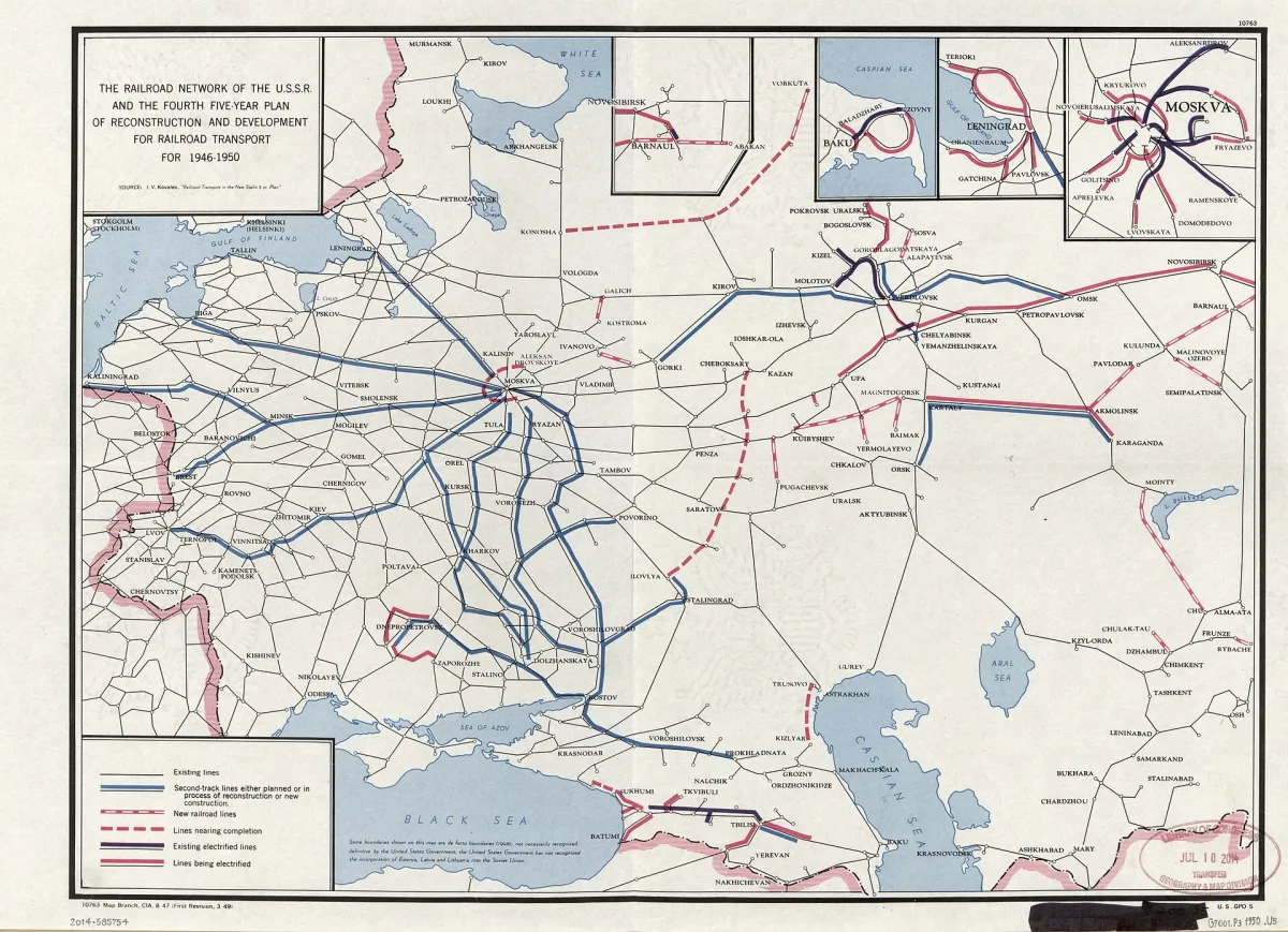
Max-flow was born applied. Ford and Fulkerson's 1956 paper records that the problem came to them from T. Harris, posed as finding the maximal steady-state flow through a railway network connecting two cities.[7] The model still runs transportation today: airlines decide which aircraft type flies which flight leg by solving flow problems on a time-expanded network whose vertices are (airport, time) pairs and whose edges are flights and ground waits. One industrial study modelled fleet assignment as a large multi-commodity flow problem with side constraints on such a network and solved real instances to within 0.02% of optimal.[8]
Cutting an object out of a photograph is, industrially, a minimum-cut computation. Build a graph with one vertex per pixel, edges between neighbouring pixels weighted by visual similarity, plus two terminals: a source standing for "object" and a sink for "background". A minimum source-sink cut then traces the cheapest boundary between the two, and it is found by computing a maximum flow, exactly the duality of this section. The method finds globally optimal boundaries efficiently and works in any number of dimensions, including 3-D medical scans.[9]
Take the cut \(S=\{s,b\}\) of Figure 6.3. Which edges count toward its capacity \(c(S,\overline{S})\)?
Why can a router that only ever adds flow along unused forward capacity stall below the maximum?
Group-valued flows: balance that wraps around
Now we return to circulations and ask the structural question: when does a graph carry a perfectly balanced flow that leaves no edge idle? Capacities disappear; the source and sink disappear; what remains is pure structure. The all-zero function is always a circulation, so the interesting demand is that the flow be nonzero on every single oriented edge.
Here the chapter widens the value system. Flow values may come from any abelian group \(H\): a set with an addition that is commutative, has a zero element, and gives every element a negative. The integers \(\mathbb{Z}\) qualify. So does clock arithmetic \(\mathbb{Z}_k\), the integers modulo \(k\), where sums wrap around (in \(\mathbb{Z}_3\), \(2+2=1\)). So do products like \(\mathbb{Z}_2\times\mathbb{Z}_3\), whose elements are pairs added coordinate by coordinate. Both defining conditions (F1) and (F2) only ever add and negate values, so they make sense over any such \(H\).
An H-flow on \(G\) is a circulation \(f:\vec{E}\to H\) that is nowhere zero: \(f(\vec{e})\neq 0\) for every oriented edge. In words: a perfectly balanced flow, valued in \(H\), that actually uses every edge of the graph.[3]
The word "flow" is overloaded, and Diestel's own footnote warns about it: much of the literature says "flow" for what this book calls a circulation, and "nowhere-zero flow" for what this book calls an H-flow. Keep the three notions apart. A circulation balances everywhere and may be zero on edges. A network flow may be unbalanced at \(s\) and \(t\) and obeys capacities. An H-flow is a circulation that avoids zero everywhere and has no capacities at all. Also beware: the sum of two H-flows need not be an H-flow, since two nonzero values can cancel on an edge.
We already know one graph property that kills every H-flow outright: a bridge, on which any circulation must vanish. So bridgeless is a necessary condition, for every group \(H\). The astonishing discovery of Tutte is how little else about \(H\) matters.
For every multigraph \(G\) there is a polynomial \(P\), the flow polynomial of \(G\), such that for every finite abelian group \(H\), the number of H-flows on \(G\) equals \(P(|H|-1)\), where \(|H|\) is the number of elements of \(H\). Consequently (Diestel, Cor. 6.3.2): two finite groups of the same size admit exactly the same answer to "does \(G\) have a flow valued here?". Only the group's size matters.[3]
The proof idea is a deletion-contraction induction: count the flows of \(G\) from the flows of \(G/e_0\) and \(G-e_0\). If every edge of \(G\) is a loop, each loop independently takes any of the \(|H|-1\) nonzero values, giving \((|H|-1)^m\) flows for \(m\) loops: a polynomial in \(|H|-1\). Otherwise pick a non-loop edge \(e_0\) and count in two pots. Circulations on \(G\) that are nonzero everywhere except possibly on \(e_0\) correspond to H-flows of the contracted graph \(G/e_0\), by the un-contract-and-patch lemma; those among them that are zero on \(e_0\), and so nonzero on every other edge, correspond to H-flows of the deleted graph \(G-e_0\). Subtract the two counts, both polynomials by induction, and the count for \(G\) is a difference of polynomials.
The 6-hour clock \(\mathbb{Z}_6\) and the pair system \(\mathbb{Z}_2\times\mathbb{Z}_3\) (a light switch coupled with a 3-hour clock) are structurally different groups, but each has exactly 6 elements. By the corollary, a graph has a \(\mathbb{Z}_6\)-flow if and only if it has a \(\mathbb{Z}_2\times\mathbb{Z}_3\)-flow. This freedom to swap groups of equal size is not a curiosity; it is a proof technique. Seymour's six-flow theorem at the end of this chapter is proved entirely inside \(\mathbb{Z}_2\times\mathbb{Z}_3\), where the two coordinates can be handled separately, and the conclusion transfers to 6 for free.
Because only size matters, one integer per graph should summarise its entire flow behaviour.
For an integer \(k\ge 1\), a k-flow is a \(\mathbb{Z}\)-flow (an integer-valued, nowhere-zero circulation) with \(0<|f(\vec{e})|<k\) on every oriented edge: allowed values \(\pm 1,\pm 2,\dots,\pm(k-1)\), never 0. The flow number \(\varphi(G)\) is the least \(k\) for which \(G\) has a k-flow, or \(\infty\) if there is none. Any k-flow is automatically an \(\ell\)-flow for every \(\ell>k\), so \(\varphi\) is a genuine threshold.[3]
"A k-flow uses the values \(1,\dots,k\)." It does not. The values are the integers of absolute value at least 1 and at most \(k-1\), with both signs. A 2-flow uses only \(\pm 1\); a 3-flow only \(\pm 1, \pm 2\). Zero is never allowed anywhere.
The flow number is the mirror image of the chromatic number. A k-colouring asks: how few colours suffice to label vertices with no conflict? A k-flow asks: how small a palette of values suffices to run a balanced, nowhere-idle flow? Both are thresholds, both are hard in general, and Section 6.5 will show they are literally two views of one quantity for graphs drawn in the plane.
Integer flows and clock-arithmetic flows might seem to live in different worlds: \(\mathbb{Z}\) is infinite, and reducing an integer flow modulo \(k\) (applying the remainder map \(\sigma_k\)) loses information. Tutte proved the worlds coincide.
A multigraph has a k-flow if and only if it has a \(\mathbb{Z}_k\)-flow.[3]
One direction is immediate: compose a k-flow with the remainder map \(\sigma_k\), and since every value has \(0<|f(\vec{e})|<k\), no value collapses to zero modulo \(k\). The other direction is the work. Start from any integer-valued function that reduces to the given \(\mathbb{Z}_k\)-flow and keeps all magnitudes below \(k\); it satisfies everything except, possibly, Kirchhoff's law. Measure its total imbalance, the sum over all vertices of \(|f(v,V)|\), and pick the candidate minimising it. If any imbalance remains, some vertex has surplus outflow. Follow edges carrying positive flow away from it; conservation forces this reachable region to contain a vertex with deficit. Push \(k\) units back along a positive walk from surplus to deficit. Because the mod-\(k\) version is balanced, every vertex's imbalance is a multiple of \(k\), so this push strictly reduces the total imbalance: contradiction. The minimiser was balanced all along, and it is a k-flow. The practical upshot: to find integer flows, it is enough to work in clock arithmetic, where flows can be built by adding partial flows without worrying about intermediate zeros.
What separates an H-flow from an ordinary circulation?
You are told that \(G\) has a 3-flow. Which statement is certain?
A gallery of small flow numbers
With the machinery in place, the natural question is concrete: which graphs have flow number 2, 3, 4? Each small value turns out to be a recognisable graph property.[4]
2-flows. Call a graph even if every vertex has even degree, where the degree \(d(v)\) counts the edge-ends at \(v\) as in Chapter 1. A graph has a 2-flow if and only if it is even (Diestel, Prop. 6.4.1). The reason fits in a breath: by Tutte's theorem just proved, a 2-flow amounts to a \(\mathbb{Z}_2\)-flow, and in \(\mathbb{Z}_2\) the only nonzero value is 1, with \(+1=-1\), so directions are irrelevant. Kirchhoff's law at a vertex then says "the number of incident edges is even". The triangle of Figure 6.1 is even, and its circulating flow used only \(\pm 1\): a 2-flow, as predicted.
3-flows on cubic graphs. A graph is cubic if every vertex has degree exactly 3, and bipartite if its vertices split into two sides with all edges running between the sides (equivalently, no odd cycle; both notions from Chapter 1). For cubic graphs: a 3-flow exists if and only if the graph is bipartite (Diestel, Prop. 6.4.2). Why: in a \(\mathbb{Z}_3\)-flow on a cubic graph, walk around any cycle; two consecutive cycle edges cannot carry the same value in the direction of travel, since the third edge at their shared vertex would then be forced to zero. So the values 1 and 2 alternate around every cycle, forcing all cycles to have even length: bipartite. Conversely, on a bipartite cubic graph, orient every edge from side \(X\) to side \(Y\) with value 1: each vertex sees three same-direction units, and \(1+1+1=0\) in \(\mathbb{Z}_3\). Balanced, nowhere zero, done. Figure 6.5 runs this construction on \(K_{3,3}\), the complete bipartite graph with three vertices on each side and all nine cross edges.
Complete graphs. Diestel writes \(K^n\) for the complete graph on \(n\) vertices (many other books write \(K_n\)). Its flow numbers form a tidy catalogue (Diestel, Prop. 6.4.3): \(\varphi(K^n)=2\) for odd \(n>1\) (all degrees even), \(\varphi(K^2)=\infty\) (a single edge is a bridge), \(\varphi(K^4)=4\), and \(\varphi(K^n)=3\) for all even \(n>4\). Two lessons hide in the list. First, \(K^4\) is the only complete graph with flow number 4: an early hint that 4 is a special, delicate value. Second, flow numbers do not grow with size or density. A complete graph on a million vertices has flow number 2 or 3. Compare colouring, where \(\chi(K^n)=n\) grows without bound: the mirror between \(\chi\) and \(\varphi\) is not an equality of difficulty everywhere, and flow numbers are conjectured to be bounded by 5 across all bridgeless graphs.
4-flows from connectivity. A graph is 4-edge-connected if at least four edges must be deleted to disconnect it. Every 4-edge-connected graph has a 4-flow (Diestel, Prop. 6.4.4). The proof borrows the tree-packing theorem from Chapter 2: 4-edge-connectivity guarantees two edge-disjoint spanning trees. Working in \(\mathbb{Z}_4\), send a unit of flow around the fundamental cycle of each non-tree edge of the first tree and add everything up; every edge outside the tree now carries \(\pm 1\). Tree edges left at zero get repaired with value-2 flows around cycles of the second tree, and a 2 can never cancel a \(\pm 1\) in \(\mathbb{Z}_4\). The sum is a nowhere-zero \(\mathbb{Z}_4\)-flow.
What a 4-flow really is. The deepest of the small-\(k\) facts uses the group \(\mathbb{Z}_2\times\mathbb{Z}_2\), legitimate because it has 4 elements, the same as \(\mathbb{Z}_4\).
(i) A graph has a 4-flow if and only if it is the union of two even subgraphs. (ii) A cubic graph has a 4-flow if and only if it is 3-edge-colourable, meaning its edges can be coloured with three colours so that no two edges sharing a vertex get the same colour.[4]
Both parts fall out of the group \(\mathbb{Z}_2\times\mathbb{Z}_2\). Its two coordinates are two independent \(\mathbb{Z}_2\)-flows, and \(\mathbb{Z}_2\)-flows are even subgraphs by Proposition 6.4.1: that is (i), a 4-flow is two overlaid 2-flows. For (ii), notice that in \(\mathbb{Z}_2\times\mathbb{Z}_2\) every element is its own negative, so orientation stops mattering and each edge carries a well-defined value among the three nonzero elements \((0,1), (1,0), (1,1)\). At a cubic vertex, two incident edges cannot share a value, or their sum would force the third edge to zero. Three edges, three distinct nonzero values: that is exactly a proper 3-edge-colouring. Conversely, the three nonzero elements sum to zero, so every 3-edge-colouring of a cubic graph is automatically balanced, hence a flow. A one-line corollary (Diestel, Cor. 6.4.6): every cubic 3-edge-colourable graph is bridgeless, since flows cannot cross bridges.
Which of these graphs has a 2-flow?
On a cubic graph, why does a proper 3-edge-colouring already behave like a 4-flow?
Flow-colouring duality: the mirror made literal
The promised mirror between colouring and flows is a theorem, and it lives in the plane. Recall from Chapter 4 that a graph drawn in the plane has a plane dual \(G^*\): one dual vertex inside each face, and one dual edge crossing each edge of \(G\). The central geometric fact carried over from that chapter is that cycles of \(G\) correspond to minimal cuts (bonds) of \(G^*\): walking a closed loop in \(G\) is the same event as severing the dual into inside and outside.
Flows are signed objects, so a bare edge-to-dual-edge dictionary is not enough; the directions must be matched too. Diestel's Lemma 6.5.1 supplies the matching: rotate each oriented edge \(\vec{e}\) clockwise onto its dual edge to get an oriented dual edge \(\vec{e}^{\,*}\), and this bijection is globally consistent, in the sense that a cycle of \(G\) traversed in one rotation corresponds to a dual cut with all its edges crossing the same way.[5] With directions matched, values transfer: given \(g\) on the dual's oriented edges, define \(f\) on \(G\)'s by \(f(\vec{e})=g(\vec{e}^{\,*})\). Diestel's Lemma 6.5.2 then characterises when the dual side is balanced: \(g\) is a circulation on \(G^*\) exactly when \(f\) obeys the sign convention and sums to zero around every cycle of \(G\), where \(f(\vec{C})\) means the sum of \(f\) along a cycle \(C\) travelled in a fixed direction.[5] Balance at every dual vertex is the same fact as cycle-balance in the original: Kirchhoff's law, reflected in the mirror.
For every dual pair \(G, G^*\) of plane multigraphs, \(\chi(G)=\varphi(G^*)\): the chromatic number of a plane multigraph equals the flow number of its dual.[5]
The proof idea is a change of viewpoint. Suppose the dual has a \(\mathbb{Z}_k\)-flow \(g\); transfer it to \(f\) on \(G\). To colour \(G\), "integrate" \(f\): pick a spanning tree with a root \(r\), give \(r\) the colour 0, and give every other vertex the \(f\)-sum along its tree path from the root. Two adjacent vertices then differ by \(\pm f\) of some edge, and \(f\) is nowhere zero, so no edge joins two same-coloured vertices: a k-colouring. Conversely, given a k-colouring \(c\), define \(f(e,v,w) = c(w)-c(v)\), the colour difference across each edge. Its values lie among \(\pm 1,\dots,\pm(k-1)\), and around any cycle the differences telescope to zero, so by the characterisation above the transferred \(g\) is a k-flow on the dual. Colourings are potentials; flows are their differences; the dual graph is where the differences live as a balanced flow.
Read the theorem's consequences in both directions. Every planar colouring statement is a flow statement about duals, so the four colour theorem of Chapter 5 becomes: every bridgeless planar multigraph has a 4-flow. And k-flows are defined for all graphs, planar or not, while plane duals exist only for plane graphs. So flow theory is what map colouring looks like once the plane is left behind, which is precisely how Tutte arrived at the conjectures of the final section. One warning to keep: the equation \(\chi(G)=\varphi(G^*)\) itself is a planar statement, since without a drawing there is no dual.
The duality proof turns a proper colouring \(c\) of a plane graph into a flow. What value does it put on the edge oriented from \(v\) to \(w\)?
The frontier: Tutte's conjectures and the six-flow theorem
Everything so far points at one question. Bridges kill flows, so bridgeless is necessary for \(\varphi(G)<\infty\). Is it sufficient, and with what bound? Tutte's answer, conjectured in 1954 and open to this day, is the oldest and most famous problem of flow theory.[6]
Every bridgeless multigraph has a 5-flow: values \(\pm 1, \pm 2, \pm 3, \pm 4\) always suffice.[6]
Via duality, the planar case is already settled: it is exactly the five colour theorem of Chapter 5, read in the mirror. The bound 5 would be best possible, because a specific small graph has flow number 5. Meet it.
A snark is a cubic bridgeless multigraph with no 4-flow, equivalently (by the two-faces theorem above) a cubic bridgeless graph that is not 3-edge-colourable. The name is borrowed from Lewis Carroll's elusive creature. The smallest snark is the Petersen graph.[6]
The Petersen graph is not just a counterexample; Tutte conjectured it is the obstruction. Recall from Chapter 1 that \(H\) is a minor of \(G\) if \(H\) arises from \(G\) by deleting and contracting. The Four-Flow Conjecture (Tutte, 1966) states: every bridgeless multigraph with no Petersen-graph minor has a 4-flow. Its planar case is the four colour theorem itself, since the Petersen graph is non-planar and so never a minor of a planar graph. For cubic graphs a proof was announced in 1998 by Robertson, Sanders, Seymour and Thomas, but the full write-up has still not appeared; the general case is open.[6] The Three-Flow Conjecture (Tutte, 1972) completes the trio: every multigraph with no one-edge cut and no three-edge cut should have a 3-flow. Its planar shadow is Grötzsch's theorem from Chapter 5, that triangle-free planar graphs are 3-colourable, and partial progress exists: Thomassen proved that sufficiently high edge-connectivity forces a 3-flow, with the requirement later brought down to 6-edge-connected.[6]
Against these open questions stands the chapter's crowning positive result.
Every bridgeless multigraph has a 6-flow. Consequently \(\varphi(G)<\infty\) if and only if \(G\) has no bridge, and the flow number of a bridgeless graph never exceeds 6.[6]
The proof in Diestel is a short 2023 argument of DeVos and Nurse, and its opening move is the group-swapping trick from earlier: since only size matters, prove a \(\mathbb{Z}_2\times\mathbb{Z}_3\)-flow. The two coordinates can then be built with different tools. The induction proves something stronger on purpose: for any chosen vertex \(u\), there is a flow whose \(\mathbb{Z}_2\)-coordinate vanishes on all edges at \(u\), a spare degree of freedom that makes the pieces glue. If deleting \(u\) leaves a bridge, split the graph along it into two contracted halves, apply induction to each, and glue, flipping the sign of one half's \(\mathbb{Z}_3\)-part if needed. If deleting \(u\) leaves a bridgeless graph, Menger's theorem from Chapter 3 supplies two edge-disjoint paths between two neighbours of \(u\); their union is a connected even subgraph, which gets contracted to a point so induction applies, and the flow is pulled back with the un-contract-and-patch lemma, routing the \(\mathbb{Z}_2\)-coordinate around the even subgraph to repair any zeros. The details are delicate, and the full account is Diestel's Section 6.6; the architecture, though, is nothing but this chapter's toolkit: group substitution, contraction lifting, and evenness as a source of 2-flows.
So the chapter closes one step short of its conjectured summit. Bridgeless graphs always carry a 6-flow; the Petersen graph shows some need 5; whether 5 always suffices has been open since 1954. Whoever started this chapter with pipes ends it facing three of the cleanest unsolved problems in graph theory, each equivalent, in the plane, to a colouring theorem from Chapter 5. The mirror between colours and flows is complete, and its far side is still being explored.
Which question does Seymour's six-flow theorem settle outright?
Check your understanding
In this chapter, what does \(\vec{E}\) stand for?
For a flow \(f\) in a network, the total value \(|f|\) is defined as:
Which values may a 3-flow assign to an oriented edge?
A graph has a 2-flow if and only if:
A cubic (3-regular) graph has a 3-flow if and only if it is:
\(f\) is a circulation on \(G\), and \(e=xy\) is a bridge. What is \(f(e,x,y)\)?
A multigraph \(G\) has an H-flow for \(H=\mathbb{Z}_6\). Which statement follows?
Why does the Petersen graph have no 4-flow?
In the network with vertices \(s, a, b, t\) and one-way capacities \(s\to a\): 2, \(s\to b\): 3, \(a\to t\): 3, \(b\to t\): 1, \(b\to a\): 1 (reverse directions 0), the maximum total flow value is:
What is the flow number \(\varphi(K^6)\) of the complete graph on six vertices?
Sources and further reading
- R. Diestel, Graph Theory, 6th ed., Springer GTM 173 (2024), §6.1 (circulations; Prop. 6.1.1, Cor. 6.1.2, Lemma 6.1.3).
- R. Diestel, Graph Theory, 6th ed., Springer GTM 173 (2024), §6.2 (networks; Prop. 6.2.1, Thm. 6.2.2, Cor. 6.2.3).
- R. Diestel, Graph Theory, 6th ed., Springer GTM 173 (2024), §6.3 (group-valued flows; Thm. 6.3.1, Cor. 6.3.2, Thm. 6.3.3).
- R. Diestel, Graph Theory, 6th ed., Springer GTM 173 (2024), §6.4 (k-flows for small k; Props. 6.4.1–6.4.5, Cor. 6.4.6).
- R. Diestel, Graph Theory, 6th ed., Springer GTM 173 (2024), §6.5 (flow-colouring duality; Lemmas 6.5.1–6.5.2, Thm. 6.5.3).
- R. Diestel, Graph Theory, 6th ed., Springer GTM 173 (2024), §6.6 and chapter notes (Tutte's conjectures, snarks; Thm. 6.6.1 with the DeVos–Nurse proof).
- L. R. Ford Jr. and D. R. Fulkerson, "Maximal Flow Through a Network", Canadian Journal of Mathematics 8 (1956), 399–404. Cambridge Core.
- C. A. Hane, C. Barnhart, E. L. Johnson, R. E. Marsten, G. L. Nemhauser and G. Sigismondi, "The fleet assignment problem: solving a large-scale integer program", Mathematical Programming 70 (1995), 211–232. Springer.
- Y. Boykov and G. Funka-Lea, "Graph Cuts and Efficient N-D Image Segmentation", International Journal of Computer Vision 70 (2006), 109–131. Springer.