Part IV · Graphs and AI
Graphs in Artificial Intelligence
Five headline AI systems, from protein folding to the model that wrote your last chatbot answer, run on graph theory you now own. This chapter shows you where the vertices and edges are hiding.
Where the graphs are hiding
You have spent twelve chapters building machinery: neighbourhoods, degrees, bipartite graphs, matchings, connectivity, planarity, flows, random graphs. This chapter leaves Diestel's book behind and asks a different question: what does modern artificial intelligence actually do with that machinery?
The answer is: more than almost any other branch of mathematics. A molecule is a graph whose vertices are atoms and whose edges are chemical bonds. A protein can be treated as a graph whose vertices are amino-acid building blocks and whose edges join the ones that sit close together in space. A road network is a weighted directed graph. A streaming service's record of who watched what is a bipartite graph. Google's index of real-world facts is a directed labelled graph with billions of edges. Even the transformer, the architecture inside large language models, can be read as a neural network operating on a complete directed graph whose vertices are the words of your sentence.
The bridge between your course and these systems is a family of models called graph neural networks. The abbreviation GNN is standard, and we will use it after this sentence: a graph neural network is a machine-learning model whose computation follows the edges of a graph. A 2024 primer in Nature Reviews Methods Primers describes GNNs as the leading approach for building predictive models on graph-structured data, with applications running from antibiotic discovery to physics simulation[1].
The plan. First we define the one operation every GNN shares, message passing, and tie it to the neighbourhood \(N(v)\) and the adjacency matrix from Chapter 1. Then we meet the three named architectures every applied paper cites. Then four readings of real systems: transformers as weighted complete digraphs, knowledge graphs as directed labelled multigraphs, recommenders as bipartite link prediction, and spectral clustering as the Laplacian matrix at work. We close with the deployed results: a new antibiotic, protein structures, faster routes in Google Maps, and a chip designed by a GNN.
One warning before we start. Nothing in this chapter is a theorem of Diestel's book. It is applied mathematics built on the book's definitions, and the citations point to the original AI papers rather than to textbook sections. Where a claim does rest on a theorem you proved, we say which chapter proved it.
This section reads a protein as a graph. What are its edges?
New notation in this chapter
Machine learning attaches numbers to vertices and edges, so we need a little notation for states, weights, and matrices. Everything else in the chapter is notation you already have.
| Symbol | Read it as | Meaning | Tiny example |
|---|---|---|---|
| \(\mathbb{R}^d\) | "R d" | The set of lists of \(d\) real numbers. A vertex state is one such list, also called a vector. | \((0.2,\,-1.5)\) is a point of \(\mathbb{R}^2\). |
| \(h_v^{(k)}\) | "the state of \(v\) after round \(k\)" | The vector of numbers vertex \(v\) carries after \(k\) rounds of message passing; \(h_v^{(0)}\) is the input data. | In Figure 13.1, \(h_b^{(0)}=2\) and \(h_b^{(1)}=8\). |
| \(H\) | "the state matrix" | The matrix whose row \(v\) is the state \(h_v\); one row per vertex. | 5 vertices with 3 numbers each: \(H\) is a \(5\times 3\) matrix. |
| \(w_{uv}\) | "the weight from \(u\) to \(v\)" | A number attached to the ordered pair \((u,v)\); an edge weight that may differ from \(w_{vu}\). | In Figure 13.2, \(w_{\text{cat},\text{sat}}=0.6\). |
| \(D\) | "the degree matrix" | The diagonal matrix with the degree \(d(v)\) in position \((v,v)\) and zeros elsewhere. | For a triangle, the diagonal reads \(2,2,2\). |
| \(L\) | "the Laplacian" | \(L = D - A\): degree matrix minus adjacency matrix. | For a triangle: \(2\) on the diagonal, \(-1\) off it. |
| \(\lambda_2\) | "lambda two" | The second-smallest eigenvalue of \(L\) (in this chapter only; it is not the edge-connectivity \(\lambda(G)\)). | \(\lambda_2 > 0\) exactly when \(G\) is connected. |
Symbols from earlier chapters get a one-clause reminder the first time they appear. The two you will see most: \(N(v)\), the neighbourhood of \(v\), meaning the set of vertices joined to \(v\) by an edge, and \(A\), the adjacency matrix, the square table with a 1 in position \((u,v)\) when \(uv\) is an edge and a 0 otherwise[2].
A graph has 6 vertices and every vertex carries a state in \(\mathbb{R}^4\). What are the dimensions of the state matrix \(H\)?
Message passing: learning on the neighbourhood
Start with the question the definition answers. Suppose each vertex of a graph carries data: for a molecule, each atom's element and charge; for a social network, each person's profile. You want a model that predicts something about a vertex, or about the whole graph, using both the data and the wiring. How should the model read a graph?
The wrong answer is to flatten the graph into a list and feed it to an ordinary neural network. A list forces you to number the vertices, and the numbering is arbitrary. You proved in Chapter 1 that a graph's essential properties are exactly the ones preserved by isomorphism, that is, by relabelling. A model that changes its answer when you relabel the input is answering a question about your bookkeeping, not about the graph.
The right answer, which the field converged on, is a protocol run by the vertices themselves.
Let \(G\) be a graph in which each vertex \(v\) holds a state \(h_v^{(k)} \in \mathbb{R}^d\). One round of message passing computes, for every vertex \(v\) at the same time, \[ h_v^{(k+1)} \;=\; f\Big( h_v^{(k)},\; \sum_{u \in N(v)} h_u^{(k)} \Big), \] where \(f\) is a small neural network whose parameters are learned from data. In words: every vertex collects the current states of its neighbours, adds them up, and feeds the total together with its own current state through a learned update function. The sum can be replaced by an average, a maximum, or a weighted sum; the shape of the protocol stays the same.
Read the formula aloud once: the new state of \(v\) is a learned function of the old state of \(v\) and the sum, over all neighbours \(u\) of \(v\), of the old states of those neighbours. The graph structure enters in exactly one place, the index set \(N(v)\) under the sum. That index set is the neighbourhood defined on the first pages of this course.
Run the round several times. After one round, \(v\) knows about its neighbours. After two rounds, its neighbours' updates already contained their neighbours, so \(v\) has information from every vertex within distance 2, where distance means the length of a shortest path, as in Chapter 1. After \(k\) rounds, \(v\) has seen exactly the vertices at distance at most \(k\): the ball of radius \(k\) around \(v\). If you want one answer for the whole graph, say "is this molecule toxic?", a final readout step pools all the vertex states into a single vector.
This framework is called the message passing neural network. It was distilled in 2017 by Gilmer and colleagues, who showed that many independently invented models for predicting molecular properties were all instances of one recipe: models that "learn a message passing algorithm and aggregation procedure to compute a function of their entire input graph"[3]. A position paper from DeepMind and collaborators the following year argued the deeper point: graphs give neural networks the right relational inductive bias, meaning the assumption, wired into the architecture, that what matters is entities and their relations, not the order in which you happen to list them[4]. Because each update reads only \(N(v)\), relabelling the vertices just relabels the outputs the same way. The model respects isomorphism by construction.
Take the graph of Figure 13.1: vertices \(a,b,c,d,e\), edges \(ab, bc, bd, ce\). Give each vertex a one-number state: \(h_a^{(0)}=1\), \(h_b^{(0)}=2\), \(h_c^{(0)}=3\), \(h_d^{(0)}=4\), \(h_e^{(0)}=5\). Run one round of the simplest possible protocol, "your new state is the sum of your neighbours' old states". Vertex \(b\) has \(N(b)=\{a,c,d\}\), so \(h_b^{(1)} = 1+3+4 = 8\). Vertex \(c\) has \(N(c)=\{b,e\}\), so \(h_c^{(1)} = 2+5 = 7\). The full result: \(2, 8, 7, 2, 3\). Note that \(d\)'s new state is 2, not 8: it uses \(b\)'s old state, because all vertices update simultaneously.
Updating vertices one after another, each reading its neighbours' already updated states. That would make the outcome depend on the order you visit the vertices, which is exactly the arbitrary bookkeeping the whole design exists to remove. Message passing is synchronous: every round-\((k{+}1)\) state is computed from round-\(k\) states only.
Now the linear-algebra reading, which is the payoff of Chapter 1's matrix section[2]. Stack the states as rows of the matrix \(H\), and let \(A\) be the adjacency matrix. Row \(v\) of the product \(AH\) is, by the definition of matrix multiplication, the sum of the rows of \(H\) over all \(u\) with \(a_{vu}=1\), that is, over all neighbours of \(v\). So the sentence "everyone sums their neighbours' states" and the formula \(H \mapsto AH\) are the same statement. In our worked example \(H\) is the column \((1,2,3,4,5)\), and \(AH = (2,8,7,2,3)\). Stacking \(k\) rounds involves \(A^k\), and the entry \((u,v)\) of \(A^k\) counts the walks of length \(k\) from \(u\) to \(v\); that is why \(k\) rounds gather information along walks of length \(k\), and why a GNN with few rounds cannot see across a graph of large diameter. Depth of network and diameter of graph are the same currency.
Message passing is structured gossip. Each round, everyone tells their friends a summary of what they currently know, and everyone folds what they hear into what they knew. After \(k\) rounds, news has travelled at most \(k\) steps. The learning part is only how each person summarizes and folds; who talks to whom is the graph, fixed and given.
Let \(G\) have edges \(ab\) and \(bc\), with states \(h_a^{(0)}=1\), \(h_b^{(0)}=2\), \(h_c^{(0)}=3\). Run one round of "your new state is the sum of your neighbours' states". What is \(h_a^{(1)}\)?
Why does the section reject flattening a graph into a numbered list and feeding it to an ordinary neural network?
Three ways to average your neighbours
Three named architectures dominate the applied literature. They differ in exactly one design choice: how the neighbourhood aggregate is computed. Knowing the three lets you read most GNN papers written since.
GCN (graph convolutional network; Kipf and Welling, 2017). The update multiplies the state matrix by a normalized adjacency matrix: each vertex takes a degree-weighted average of its neighbours' states, plus its own after a loop is added at every vertex, then applies a learned linear map. The authors derived the rule as "a localized first-order approximation of spectral graph convolutions"[5]: it began life in the spectral theory of the Laplacian, which we meet later in this chapter, and was simplified until only a cheap local averaging step survived. The normalization matters. Without division by degree, the states of high-degree vertices grow with every round and drown out the rest; the fix is dictated by the degree sequence, a Chapter 1 object.
GAT (graph attention network; Veličković and colleagues, 2018). Instead of fixed degree-based weights, GAT learns how much each neighbour matters. For each edge \(uv\), a small network scores how relevant \(u\)'s state is to \(v\); the scores across \(N(v)\) are scaled to be positive and sum to 1, and \(v\) takes the weighted average[6]. In graph language: GAT converts the input graph into a weighted graph whose weights \(w_{uv}\) are computed from the data, fresh at every layer. This helps when neighbourhoods are mixed in quality; in a citation network, some references matter far more than others.
GraphSAGE (Hamilton, Ying, and Leskovec, 2017). The scalability workhorse, with two changes. First, instead of using all of \(N(v)\), it samples a fixed number of neighbours, say 25, so the cost per vertex stays bounded even at a vertex of enormous degree. Second, it is trained to be inductive: it learns the aggregation function itself, not a separate stored vector per vertex, so it can "efficiently generate node embeddings for previously unseen data"[7]. Earlier methods were transductive: they memorized one fixed graph and had no answer for a vertex that arrived after training. With GraphSAGE, a user who signs up tomorrow is embedded immediately from their features and neighbourhood. This is the design change that made GNNs deployable on industrial graphs, as we will see at Pinterest below.
Two course connections. The sampled neighbourhoods of GraphSAGE are random subgraphs of the ball around \(v\), so its guarantees are statements about random subgraph approximation, kin to the probabilistic arguments of Chapter 11. And the random graph model of that chapter, independent edges with equal probability, is a useful foil here: real social and interaction graphs violate it dramatically, with heavy-tailed degree sequences and dense clustering, and all three architectures carry design scars from those violations, from GCN's normalization to GraphSAGE's sampling.
In a citation network some references matter far more than others. Which of the three architectures is designed for that, and how?
Transformers: attention is a weighted complete digraph
The transformer is the architecture inside GPT-style language models, introduced in the 2017 paper "Attention Is All You Need"[8]. Its core operation, self-attention, works like this. Every token, roughly a word piece, holds a vector. To update itself, a token computes a compatibility score with every token in the sentence, converts the scores into positive weights that sum to 1, and takes the weighted average of all the tokens' vectors.
Now read that paragraph as a graph theorist. Take the tokens as the vertex set. Every vertex aggregates from every other vertex, so the "neighbourhood" is all of \(V\): the underlying graph is the complete graph \(K^n\) on the \(n\) tokens, every pair joined, plus a loop at each vertex because a token attends to itself. The attention weights are edge weights. And since the weight token \(i\) gives to token \(j\) need not equal the weight \(j\) gives to \(i\), the right object is a weighted complete directed graph: \(n(n-1)\) ordered pairs, each carrying its own learned weight \(w_{ij}\), recomputed for every input at every layer.
This is not a loose analogy. Chaitanya Joshi's widely read essay "Transformers are Graph Neural Networks" makes it precise: a transformer is a GNN that treats a sentence as "a fully-connected graph, where each word attends to every other word", with multi-head attention as the neighbourhood aggregation function[9]. The two research communities reached the same update rule from opposite directions, and a graph attention network that happens to run on a complete graph is, in all but bookkeeping, a transformer layer[9].
Assuming attention is symmetric. The weight "sat" gives to "cat" and the weight "cat" gives to "sat" are computed separately and generally differ, so the structure is a digraph, not a graph. If you model it with an undirected weighted \(K^n\) you have thrown away half the numbers.
Two refinements complete the picture. First, causal masking as orientation. In a decoder, the GPT setting, each token may only attend to earlier tokens. In graph terms you have oriented the complete graph by the token order: every arc points from an earlier token to a later one. An orientation of a complete graph by a linear order has no directed cycles, and that acyclicity is what lets generation proceed left to right, one token at a time. Second, positional encodings as graph repair. A complete graph on tokens has forgotten the word order; every vertex looks the same, which is precisely the isomorphism-invariance that helps molecules and hurts sentences. Transformers restore order by adding position information to each token's input vector[8]. On general graphs the analogous trick is to give each vertex coordinates derived from the graph's structure, and a standard choice is eigenvectors of the Laplacian, the matrix we are about to meet.
One more line worth writing down. The famous cost of attention, quadratic in the sentence length, is a statement you can prove: \(\|K^n\| = \binom{n}{2} = n(n-1)/2\), the size (number of edges) of the complete graph, doubled for direction. The engineering bottleneck of large language models is the edge count of \(K^n\) wearing a compute budget.
In Figure 13.2 the weight "cat" gives to "sat" is 0.6. In a self-attention layer with no causal mask, what does that tell you about the weight "sat" gives to "cat"?
A sentence has 50 tokens. Ignoring the self-loops, how many attention weights does one unmasked self-attention layer compute?
Knowledge graphs: facts as labelled arcs
How should a machine store the fact that Marie Curie won the Nobel Prize in Physics? Not as a sentence, which is hard to query, and not as a rigid database table, which fixes in advance what kinds of facts exist. The answer that won: store facts as edges of a graph.
A knowledge graph is a directed graph whose vertices are entities (people, places, proteins, products) and whose arcs carry labels naming relations. Its atomic unit is the triple (subject, predicate, object), such as (Marie Curie, won, Nobel Prize in Physics): a directed labelled arc from the subject vertex to the object vertex. Plainly: a fact is an arrow with a name on it.
The standard exchange format for such data on the web is RDF, the Resource Description Framework, a W3C standard, and its primer states the graph reading outright: triples form a directed labelled graph in which subjects and objects become vertices while predicates form the connecting arcs[10]. Since two entities can be linked by several differently labelled arcs, and direction carries meaning, the honest classification in course language is: a directed multigraph with labelled arcs, the objects Chapter 1 defined in its closing sections[2]. A survey by Hogan and seventeen co-authors frames knowledge graphs as the tool of choice for "diverse, dynamic, large-scale collections of data" where a fixed schema fits badly[11].
The deployment that named the concept: in 2012 Google announced its Knowledge Graph under the slogan "things, not strings", arguing that search should understand entities and their relationships rather than match keywords. At launch it held more than 500 million objects and more than 3.5 billion facts about the relationships between them[12]. In course terms, a directed labelled graph with 3.5 billion arcs, powering the information boxes beside search results.
Where the machine learning enters: real knowledge graphs are incomplete. A core task is link prediction, guessing which absent arcs are probably true, done with GNNs or by placing each vertex and each relation label into \(\mathbb{R}^d\) and scoring candidate triples geometrically[11]. And querying is your Chapter 1 material wearing a suit: "which actors starred in films directed by someone born in Lisbon?" is pattern matching over directed walks, multi-hop reasoning is path-following, and whether an answer is reachable at all is a question about directed connectivity, the concern of Chapter 3. Knowledge graphs also anchor today's language models: retrieval systems walk the graph to fetch verified facts for the model to put into words[11].
Why does the chapter classify a knowledge graph as a directed multigraph with labelled arcs rather than a plain directed graph?
Recommenders: link prediction on bipartite graphs
Recommendation data is a bipartite graph by birth. One vertex class for users, one for items, an edge exactly when a user watched, bought, or rated an item, and no edges inside a class. That is the structure Diestel defines in Section 1.6, and you know its signature theorem: a graph is bipartite if and only if it contains no odd cycle[2]. The matching theory of Chapter 2, König's theorem and Hall's marriage condition, lives on exactly this class of graphs[13]: assigning items to users under constraints is a bipartite matching problem, and a recommender can be read as the machine that produces the weighted preferences such an assignment would optimize over.
What does a recommender actually compute? A prediction about missing edges. "You might like this film" means: the model believes the edge between your vertex and the film's vertex is absent from the data but present in the truth. Recommendation is link prediction on a bipartite graph, and the signal travels along walks: user \(u\) liked item \(m\), other users liked \(m\), those users liked further items, which become candidates for \(u\). Every such walk alternates sides, a fact you proved when you characterized bipartite graphs by their cycles.
Two verified landmarks show the scale this runs at. PinSage, published by Pinterest and Stanford in 2018, put GraphSAGE-style ideas into production on a graph of 3 billion vertices and 18 billion edges. Full neighbourhoods are unmanageable at that size, so PinSage "combines efficient random walks and graph convolutions": it defines a vertex's effective neighbourhood by short random walks and aggregates over the most-visited vertices[14]. This was the demonstration that GNNs work at web scale. LightGCN, from 2020, ran the opposite direction: strip the GCN down. It "learns user and item embeddings by linearly propagating them on the user-item interaction graph", removing the learned nonlinear transforms entirely, and beat heavier models on standard benchmarks[15]. The lesson for a graph theory student is satisfying: on a bipartite interaction graph, most of the predictive power is in the graph structure itself. Propagation along the edges does the work.
In the user-item graph, the recommendation signal travels along walks. A walk that starts at a user vertex and ends at a user vertex must have:
The Laplacian goes to work
The question first: given data points with no labels, how do you find the natural groups? The most graph-theoretic answer in machine learning is spectral clustering, and its engine is one matrix.
Let \(G\) be a graph on \(n\) vertices, \(A\) its adjacency matrix, and \(D\) the diagonal matrix carrying the degrees \(d(v)\). The Laplacian of \(G\) is \(L = D - A\). Plainly: row \(v\) of \(L\) has the degree of \(v\) on the diagonal, a \(-1\) in the column of every neighbour of \(v\), and zeros elsewhere. Each row sums to zero, because a degree is exactly a count of neighbours.
An eigenvector of a square matrix \(M\) is a nonzero vector \(x\) that \(M\) merely stretches: \(Mx = \lambda x\) for some number \(\lambda\), called its eigenvalue. Plainly: a direction the matrix does not turn, only scale. For the Laplacian we list the eigenvalues in increasing order \(\lambda_1 \le \lambda_2 \le \dots \le \lambda_n\).
Notation clash: in Chapter 1, \(\lambda(G)\) is the edge-connectivity of \(G\), the least number of edges whose deletion disconnects it. In the spectral literature, and in this chapter from here on, \(\lambda_i\) is the \(i\)-th smallest eigenvalue of \(L\). The two uses are related in spirit (both measure how robustly connected a graph is) but they are different numbers. Read \(\lambda\) by context.
The Laplacian stores a startling amount of the graph in its eigenvalues. Three facts, in increasing order of usefulness. First, \(L\) is symmetric and all its eigenvalues are at least 0. Second, 0 is always an eigenvalue: apply \(L\) to the all-ones vector, and each row sums to zero, so the result is the zero vector. Third, and this is the theorem of the section:
For any graph \(G\), the multiplicity of the eigenvalue 0 of the Laplacian \(L\) equals the number of connected components of \(G\)[16]. In particular, \(\lambda_2 > 0\) exactly when \(G\) is connected.
Proof idea. The computation that unlocks everything is the identity \(x^{\top} L x = \sum_{uv \in E} (x_u - x_v)^2\): the Laplacian measures how much a vertex-labelling \(x\) disagrees across edges. If \(Lx = 0\) then that sum of squares is zero, so \(x\) is constant along every edge, hence constant on each connected component (walk along a path, as in Chapter 1, and the value never changes). So the vectors with \(Lx=0\) are exactly the ones built by choosing one constant per component, and there are as many independent choices as components. The full argument is short linear algebra; von Luxburg's tutorial gives it in one page[16].
Connectivity, a qualitative Chapter 1 notion, has become a number you can compute by matrix algebra. The refinement is where machine learning lives: for a connected graph, \(\lambda_2\) measures how close the graph is to disconnecting, and the eigenvector belonging to \(\lambda_2\), called the Fiedler vector, assigns each vertex a real number. Sorting or thresholding those numbers tends to split the graph along a sparse cut: few edges crossing, both sides substantial[16].
Spectral clustering turns this into an algorithm for arbitrary data. Build a similarity graph on your data points, connecting each point to its nearest neighbours. Compute the first \(k\) eigenvectors of the Laplacian, which hands every vertex \(k\) coordinates. Then run a simple geometric grouping method (\(k\)-means) in that \(k\)-dimensional space. Von Luxburg's 2007 tutorial is the standard reference; it lays out the Laplacian variants and why the method finds cluster structure that purely geometric methods miss[16]. The reason the eigenvector shows up at all is a relaxation story. The natural cut-quality objectives are computationally hard to optimize exactly, because they ask for a cut that is also balanced, and a plain minimum cut is not; allow each vertex any real number instead of a hard \(+1\) or \(-1\), and the optimization becomes an eigenvector computation whose answer is the Fiedler vector[16]. Cuts, you may recall, are the dual objects of flows, and the max-flow min-cut theorem of Chapter 6 is the exact-combinatorics counterpart of what this relaxation solves approximately[17].
Spectral ideas thread through the rest of the chapter's cast. The GCN layer began as a spectral filter and was simplified to local averaging[5]. Graph transformers attach the first few Laplacian eigenvector values to each vertex as position coordinates, the graph-world analogue of the positional encodings in the original transformer. And a small \(\lambda_2\) warns of a bottleneck: when much information must cross a sparse cut in few message-passing rounds, it gets compressed too aggressively, a failure GNN researchers call over-squashing.
A graph on 6 vertices consists of a triangle together with a disjoint path on the other 3 vertices. How many times does 0 occur as an eigenvalue of its Laplacian \(L\)?
Figure 13.5 shows two dense clusters joined by just two edges. What does the section say about \(\lambda_2\) and its eigenvector here?
Molecules: AlphaFold and a new antibiotic
Now the deployed systems, starting with the smallest graphs and the biggest headlines.
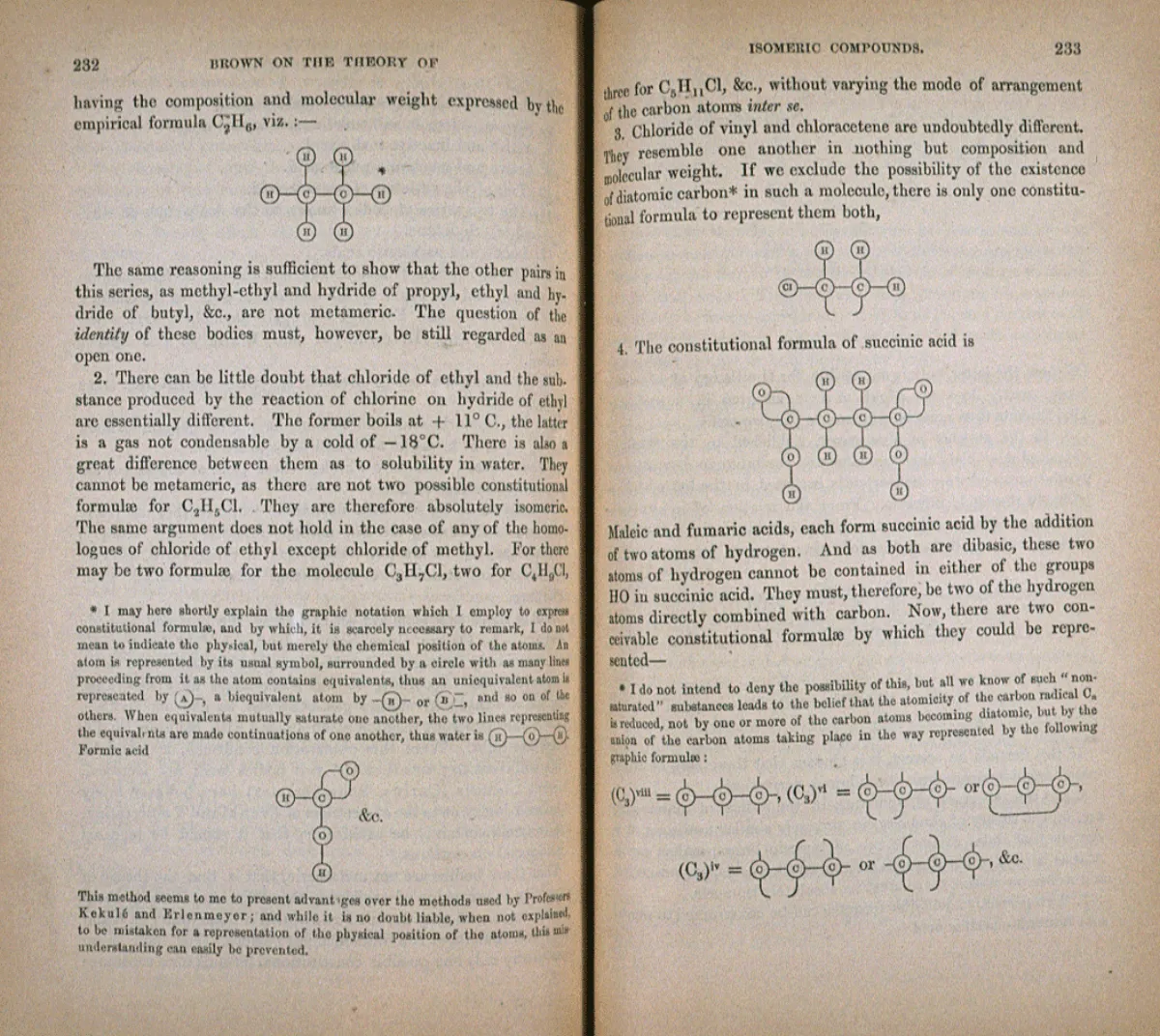
A molecule is a graph you can hold: atoms as vertices, bonds as edges. Figure 13.6 draws ethanol, the alcohol in wine, whose molecular graph has nine vertices and eight edges. It is a tree, which you can verify by counting: nine vertices, eight edges, connected, no cycle.
Feed graphs like this, with atom data as vertex states, into a message-passing network, and you get a molecular property predictor; this was precisely the setting in which the message-passing framework was distilled[3]. The result that made the approach famous came in 2020. A team at MIT trained a deep model of exactly this type on roughly 2,500 molecules labelled by whether they inhibit the growth of E. coli, then screened large chemical libraries in software[18]. The model surfaced a molecule the team named halicin, which killed many antibiotic-resistant bacteria in laboratory and animal tests, including strains resistant to all known antibiotics[19]. Halicin is structurally unlike existing antibiotics, and that is the point: the network judged molecules by learned structural features of the graph, not by resemblance to known drugs[19].
The sequel made the graphs visible. In 2023, Wong, Zheng and colleagues trained ensembles on 39,312 experimentally screened compounds, predicted antibiotic activity across 12 million molecules, and then used explainable models to identify which chemical substructures drive the predictions. A substructure of a molecule is a subgraph of its molecular graph. The search produced a new structural class of antibiotics active against MRSA, the methicillin-resistant staph bacterium, validated in mouse models[20]. The model's evidence for its own prediction is a distinguished subgraph.
Proteins scale the same idea up. AlphaFold, from DeepMind, predicts a protein's three-dimensional shape from its chain of amino acids, with accuracy competitive with laboratory experiment for most proteins; the 2021 Nature paper is among the most cited scientific papers of its decade[21]. The graph content is explicit in the paper, which treats "the prediction of protein structures as a graph inference problem in 3D space in which the edges of the graph are defined by residues in proximity"[21]. Alongside a per-residue representation, the network maintains a feature vector for every ordered pair of residues: learned edge features on a complete digraph over the residues, iteratively refined so that geometry becomes consistent (if residue \(A\) sits near \(B\), and \(B\) near \(C\), the \(A\)-\(C\) edge feature must be compatible). Here is the course-language summary. The amino-acid sequence hands you a path graph, the barest connected graph there is. Folding is the discovery of the rest of the edge set.
Ethanol's molecular graph has 9 vertices, 8 edges, and is connected. What follows at once?
Maps and chips
Routing is the classical graph story: model the road network as a directed graph, one vertex per intersection or road segment, weight each arc by travel time, and run a shortest-path algorithm. Distance and shortest paths are Chapter 1; nothing about the algorithmic frame changed. What deep learning changed is the weights. Travel time is not a constant; it is a prediction problem that depends on traffic now and twenty minutes from now.
In 2020, DeepMind and Google Maps put GNN-based travel-time prediction into production, improving the accuracy of estimated arrival times by up to 50% in cities including Berlin, Jakarta, São Paulo, Sydney, Tokyo, and Washington, D.C.[22] The accompanying paper explains the method: the road network is carved into "supersegments", connected chains of road segments treated as graphs on which a GNN predicts traversal times, capturing how congestion spreads along adjacent segments; deployment cut severe mispredictions by more than 40% in cities like Sydney[23].
Why must travel times be predicted jointly rather than one segment at a time? Because traffic is a flow on the network, in the sense of Chapter 6: what enters a segment must have left its neighbours, so congestion couples adjacent arcs, and delays pile up near saturated cuts. A GNN passing messages along the road graph is learning exactly those couplings. The final step is untouched theory: once the weights are set, the route you are shown is still a shortest path.
The last stop is the hardware itself. Chip floorplanning is the task of deciding where each block of circuitry sits on the silicon die. The input is a netlist: a graph of circuit components and the wires connecting them (strictly, a hypergraph, since one wire can join several components). In 2021, Mirhoseini, Goldie and colleagues published in Nature a method that treats floorplanning as a game played by a learning agent, in which "an edge-based graph convolutional neural network" reads the netlist and guides the placement of components one by one, producing layouts in under six hours that match or beat expert human designers on power, performance, and area[24]. Google later confirmed that the method, now called AlphaChip, produced layouts used in three consecutive generations of its Tensor Processing Units, the v5e, v5p, and Trillium chips that train and serve its AI models[25]. There is a pleasing loop here: a graph neural network designs the hardware that runs graph neural networks.
The course connection runs through Chapter 4. A netlist must be realized on an essentially two-dimensional surface, and real netlists are nowhere near planar, which is why chips route wires across a limited number of stacked layers and why crossing-minimization intuition applies. Placement quality is scored partly by total wirelength, which is a property of the drawing, not of the abstract graph; the distinction between a graph and its drawing, which Chapter 4 made precise, is exactly the distinction AlphaChip's score function lives on.
What did the graph neural network change about the way Google Maps produces a route?
What to keep
One idea organizes this whole chapter. Modern AI did not import graph theory as decoration; it rediscovered the subject's central discipline, which is to compute only with structure that survives relabelling. Message passing is the neighbourhood \(N(v)\) made executable. Attention is a weighted \(K^n\) with directions. A knowledge graph is a directed labelled multigraph with a query language. A recommendation is a predicted edge in a bipartite graph. Spectral clustering is connectivity, differentiated. When you meet the next AI system, the useful first question is the one this course has trained you to ask: what are the vertices, what are the edges, and which of its properties are isomorphism-invariant?
If you want to go deeper on the AI side, the four best entry points among this chapter's sources are the message-passing paper[3], the relational inductive bias position paper[4], Joshi's transformer essay[9], and von Luxburg's spectral clustering tutorial[16]. All four are readable with what you now know.
This section names the one discipline of graph theory that modern AI rediscovered. Which is it?
Check your understanding
In one round of message passing (before any neighbour sampling), a graph neural network computes the new state of vertex \(v\) from the old states of exactly which vertices?
Stack the one-number vertex states of a graph into a column \(H\), and let \(A\) be the adjacency matrix. The round "every vertex's new state is the sum of its neighbours' old states" is the same computation as which matrix product?
After \(k\) rounds of message passing, the state of vertex \(v\) can depend on the input data of which vertices?
GraphSAGE is called inductive. What does that buy in practice?
Viewing a transformer's self-attention layer (no causal mask) through graph theory, the tokens and their attention weights form which structure?
In a GPT-style decoder, each token may attend only to earlier tokens. In graph terms, this causal mask turns the attention structure into:
An RDF triple such as (Turing, born in, London) corresponds to which object in a knowledge graph?
A movie service models its data with a vertex per user, a vertex per movie, and an edge exactly when a user rated a movie. Which statement about this graph is guaranteed?
Let \(L = D - A\) be the Laplacian of a graph \(G\). The multiplicity of the eigenvalue 0 of \(L\) equals:
The GCN update divides each aggregated neighbour sum by (roughly) the vertex degrees. What problem does this normalization address?
Sources and further reading
- G. Corso, H. Stark, S. Jegelka, T. Jaakkola, R. Barzilay, "Graph neural networks", Nature Reviews Methods Primers 4, 17 (2024). nature.com/articles/s43586-024-00294-7.
- R. Diestel, Graph Theory, 6th ed., Springer GTM 173 (2024), §1.2 (degrees), §1.6 (bipartite graphs and the odd-cycle characterization, Prop. 1.6.1), §1.9 (the adjacency matrix), §1.10 (directed graphs and multigraphs).
- J. Gilmer, S. S. Schoenholz, P. F. Riley, O. Vinyals, G. E. Dahl, "Neural Message Passing for Quantum Chemistry" (2017). arXiv:1704.01212.
- P. W. Battaglia, J. B. Hamrick, V. Bapst, et al., "Relational inductive biases, deep learning, and graph networks" (2018). arXiv:1806.01261.
- T. N. Kipf, M. Welling, "Semi-Supervised Classification with Graph Convolutional Networks", ICLR 2017. arXiv:1609.02907.
- P. Veličković, G. Cucurull, A. Casanova, A. Romero, P. Liò, Y. Bengio, "Graph Attention Networks", ICLR 2018. arXiv:1710.10903.
- W. L. Hamilton, R. Ying, J. Leskovec, "Inductive Representation Learning on Large Graphs", NIPS 2017. arXiv:1706.02216.
- A. Vaswani, N. Shazeer, N. Parmar, J. Uszkoreit, L. Jones, A. N. Gomez, L. Kaiser, I. Polosukhin, "Attention Is All You Need" (2017). arXiv:1706.03762.
- C. K. Joshi, "Transformers are Graph Neural Networks", The Gradient (2020). thegradient.pub/transformers-are-graph-neural-networks.
- W3C, RDF 1.1 Primer, W3C Working Group Note, 24 June 2014. w3.org/TR/rdf11-primer.
- A. Hogan, E. Blomqvist, M. Cochez, et al., "Knowledge Graphs", ACM Computing Surveys 54(4) (2021). arXiv:2003.02320.
- A. Singhal, "Introducing the Knowledge Graph: things, not strings", Google Official Blog, May 16, 2012. blog.google/products/search/introducing-knowledge-graph-things-not.
- R. Diestel, Graph Theory, 6th ed., Springer GTM 173 (2024), §2.1 (König's theorem 2.1.1; Hall's marriage theorem 2.1.2).
- R. Ying, R. He, K. Chen, P. Eksombatchai, W. L. Hamilton, J. Leskovec, "Graph Convolutional Neural Networks for Web-Scale Recommender Systems", KDD 2018. arXiv:1806.01973.
- X. He, K. Deng, X. Wang, Y. Li, Y. Zhang, M. Wang, "LightGCN: Simplifying and Powering Graph Convolution Network for Recommendation", SIGIR 2020. arXiv:2002.02126.
- U. von Luxburg, "A Tutorial on Spectral Clustering", Statistics and Computing 17(4) (2007). arXiv:0711.0189.
- R. Diestel, Graph Theory, 6th ed., Springer GTM 173 (2024), §6.2 (the max-flow min-cut theorem 6.2.2).
- J. M. Stokes, K. Yang, K. Swanson, W. Jin, A. Cubillos-Ruiz, et al., "A Deep Learning Approach to Antibiotic Discovery", Cell 180 (2020). doi.org/10.1016/j.cell.2020.01.021.
- A. Trafton, "Artificial intelligence yields new antibiotic", MIT News, February 20, 2020. news.mit.edu/2020/artificial-intelligence-identifies-new-antibiotic-0220.
- F. Wong, E. J. Zheng, et al., "Discovery of a structural class of antibiotics with explainable deep learning", Nature 626 (2023). nature.com/articles/s41586-023-06887-8.
- J. Jumper, et al., "Highly accurate protein structure prediction with AlphaFold", Nature 596 (2021). nature.com/articles/s41586-021-03819-2.
- Google DeepMind, "Traffic prediction with advanced Graph Neural Networks", DeepMind blog, September 3, 2020. deepmind.google/discover/blog/traffic-prediction-with-advanced-graph-neural-networks.
- A. Derrow-Pinion, J. She, D. Wong, et al., "ETA Prediction with Graph Neural Networks in Google Maps", CIKM 2021. arXiv:2108.11482.
- A. Mirhoseini, A. Goldie, M. Yazgan, et al., "A graph placement methodology for fast chip design", Nature 594 (2021). nature.com/articles/s41586-021-03544-w.
- Google DeepMind, "How AlphaChip transformed computer chip design", DeepMind blog, September 26, 2024. deepmind.google/discover/blog/how-alphachip-transformed-computer-chip-design.