Part III · The Deep Theory
Chapter 8: Infinite Graphs
Every graph so far had finitely many dots and lines. This chapter lets a graph run on forever, teaches the three proof tools that keep infinity under control, and introduces something genuinely new: the ends of a graph, its points at infinity.
What changes when a graph never ends
Picture the natural numbers \(0, 1, 2, 3, \ldots\) as dots, with a line between each number and the next. Or picture the street corners of a city whose grid of streets extends forever north and forever east. These are perfectly ordinary graphs in the sense of Chapter 1: a set of vertices, a set of edges, each edge joining two vertices. Nothing in the definition ever said the sets had to be finite.
Almost all the vocabulary survives unchanged: degrees, paths, trees, connectedness, colourings all mean what they meant before. What changes is the reasoning. A finite argument often works by repeating a step until the vertices run out; in an infinite graph they never do, and a construction that looks fine at every step can still produce garbage in the limit. The first half of this chapter teaches the three standard tools that repair this: Zorn's lemma, transfinite induction, and compactness. The second half is about a concept with no finite counterpart at all: the ends of a graph, the distinct directions in which one can walk to infinity.
Two pieces of vocabulary first. Throughout the chapter, "countable" means finite or as large as the set \(\mathbb{N}\) of natural numbers, and \(\aleph_0\) (read "aleph-nought") is the size of \(\mathbb{N}\): the smallest infinite size. The complete graph on countably many vertices is written \(K^{\aleph_0}\). (Diestel writes complete graphs with a superscript, \(K^n\) and \(K^{\aleph_0}\); many other books write \(K_n\).)
A ray is a one-way infinite path: vertices \(x_0, x_1, x_2, \ldots\), all distinct, with edges \(x_0x_1, x_1x_2, x_2x_3, \ldots\) A double ray is the two-way version, with vertices \(\ldots, x_{-1}, x_0, x_1, \ldots\) A tail of a ray is what remains after deleting a finite initial piece: for example \(x_5 x_6 x_7 \ldots\) is a tail of \(x_0 x_1 x_2 \ldots\) In plain words: a ray is a path that walks off to infinity in one direction, a double ray walks off in both, and any two tails of a ray agree except for a finite start.
A graph is locally finite if every vertex has finite degree, where the degree \(d(v)\) is, as always, the number of edges at the vertex \(v\). In plain words: no single vertex touches infinitely many edges, so infinity can only come from having infinitely many vertices. The ray and the endless street grid are locally finite; the infinite star (one hub joined to infinitely many tips) is not.
Local finiteness separates the two kinds of infinity a graph can have: being infinitely long (containing rays) and being infinitely wide (containing a vertex of infinite degree). Most of the cleanest theory in this chapter, especially the topological second half, is about locally finite graphs, where only the "long" kind occurs.
"Infinite just means very large, so limits of good steps are good." No. The sets \(A_n = \{n, n+1, n+2, \ldots\}\) are infinite and nested, yet their common intersection is empty: every number \(m\) is missing from \(A_{m+1}\). The same trap catches graph constructions: a process can be harmless at every finite stage and still destroy what you wanted at the limit. The chapter's core skill is recognizing when limits are safe (when the forbidden object, like a cycle, is finite and would already appear at some finite stage) and when they are not (when the forbidden object, like a ray, can materialize only at the limit).
Which of these infinite graphs is locally finite?
New notation in this chapter
Three symbols get recycled with new meanings here, so read this table carefully: in this chapter \(|G|\) and \(\|G\|\) are topological spaces (not the order and size of \(G\) from Chapter 1), and the letter \(\omega\) names an end (not the clique number).
| Symbol | Read it as | Meaning | Tiny example |
|---|---|---|---|
| \(\aleph_0\) | "aleph-nought" | The smallest infinite cardinal: the size of \(\mathbb{N}\); "countably infinite." | The ray has \(\aleph_0\) vertices. |
| \(K^{\aleph_0}\) | "K aleph-nought" | The complete graph on countably infinitely many vertices. | Any two of its vertices are adjacent. |
| \(TX\) | "a subdivision of X" | A copy of the graph \(X\) with each edge possibly replaced by a longer path. | Replacing every edge of a triangle by a 2-edge path gives a \(TK^3\). |
| \(\omega\) | "an end omega" | An end: an equivalence class of rays that no finite vertex deletion can separate. | All rays of the infinite grid form one end. |
| \(\Omega(G)\) | "the ends of G" | The set of all ends of \(G\); one also writes \(G = (V, E, \Omega)\). | For the double ray, \(|\Omega| = 2\). |
| \(T_2\) | "the binary tree" | The rooted tree whose vertices are the finite 0–1 strings; each string \(s\) has upper neighbours \(s0\) and \(s1\). | Vertex \(01\) has upper neighbours \(010\) and \(011\). |
| \(H^\infty\) | "the hexagonal quarter grid" | A brick-wall-patterned subgraph of the infinite grid; every vertex has degree at most 3. | Halin's grid theorem finds a \(TH^\infty\) in any graph with a thick end. |
| \(nH\), \(\aleph_0 H\) | "n copies of H" | The disjoint union of \(n\), respectively countably many, copies of \(H\). | \(3K^3\) is three disjoint triangles. |
| \(R\) | "the Rado graph" | The unique countable graph with the extension property \((\ast)\). | Deleting finitely many vertices of \(R\) leaves a copy of \(R\). |
| \((\ast)\) | "the extension property" | For any disjoint finite vertex sets \(U, W\) some vertex is adjacent to all of \(U\) and none of \(W\). | Used back-and-forth to prove \(R\) unique. |
| \(|G|\) | "the space of G" | The topological space made of \(G\) plus its ends (Section 8.6). Not the order of \(G\) in this chapter. | For \(G\) a ray, \(|G|\) is a closed interval. |
| \(\mathring e\), \(\overline X\) | "the interior of e; the closure of X" | \(\mathring e\): the inside of edge \(e\), without its endpoints; \(\overline X\): the point set \(X\) plus all points it approaches in \(|G|\). | \(\overline V = V \cup \Omega\). |
| arc, circle, circuit | — | Arc: a topological copy of the segment \([0,1]\) inside \(|G|\); circle: a topological copy of the round circle; circuit: the edge set of a circle. | A double ray plus its two distinct ends is an arc. |
| \(\mathcal{C}(G)\) | "the topological cycle space" | All thin sums of circuits, finite or infinite (Section 8.7). | Both rails of the ladder plus one rung form a member. |
| \(\mathcal{C}_{\text{fin}}(G)\) | "the finitary cycle space" | Finite sums of finite circuits, as in Chapter 1. | \(\mathcal{C}_{\text{fin}}(G) \subseteq \mathcal{C}(G)\); the inclusion is proper as soon as \(G\) has an infinite circuit, as the ladder does. |
| \(C_e\), \(D_f\) | "fundamental circuit; fundamental cut" | For a topological spanning tree: the unique circuit through chord \(e\); the set of edges joining the two pieces of the tree minus \(f\). | \(e \in D_f\) exactly when \(f \in C_e\). |
| \(G/p\) | "G contracted by p" | The finite multigraph obtained by collapsing each class of a finite vertex partition \(p\) to a single vertex. | Collapsing all of \(G\) minus a finite set, component by component. |
| \(\|G\| = \varprojlim |G/p|\) | "the inverse limit" | The space of all consistent choices of one point in every finite view \(|G/p|\). Not the size of \(G\) in this chapter. | Theorem: \(\|G\| \cong |G|\) for connected locally finite \(G\). |
In this chapter, what does the symbol \(|G|\) stand for?
Three tools for taming infinity
Why do we need new tools at all? Take the most innocent statement imaginable: every connected graph has a spanning tree, a cycle-free connected subgraph containing every vertex. The finite proof grows the tree one vertex at a time and stops when the vertices are used up. In an infinite graph that procedure never stops, so the proof says nothing. The statement is still true[1], but each of its proofs demonstrates one of the chapter's tools.
Tool 1: Zorn's lemma. Instead of building the object step by step, grab a maximal one all at once. Zorn's lemma says: in a partially ordered collection, if every chain (totally ordered sub-collection) has an upper bound in the collection, the collection has a maximal element. For spanning trees, order all trees inside \(G\) by inclusion. A chain of trees has an upper bound, its union: any cycle in the union would be finite, hence would already lie inside one single tree of the chain. Zorn hands us a maximal tree, which must reach every vertex (a missed vertex adjacent to the tree could be added). Note where finiteness of cycles did the real work: it made the limit safe.
Tool 2: transfinite induction. Keep the step-by-step construction, but let it continue past infinity, with ordinal numbers as the clock: after steps \(0, 1, 2, \ldots\) comes a limit step, then further steps beyond it. At ordinary steps you add a vertex; at limit steps you take the union of everything so far, and again finiteness of cycles makes the unions safe. The formal machinery of ordinals lives in Diestel's Appendix A[9]; the mental picture "step-by-step, with union steps sprinkled in" is enough for this course.
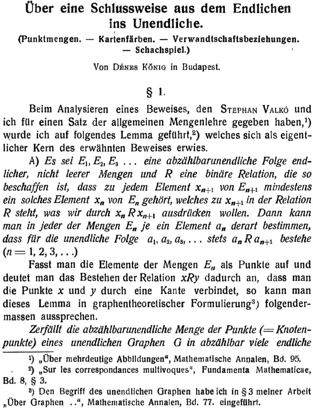
Tool 3: compactness. Solve the problem on every finite piece, then glue the finite solutions into one infinite solution. This is the tool with the biggest payoff, and its graph-theoretic engine is a lemma of Dénes Kőnig.
Let \(V_0, V_1, V_2, \ldots\) be disjoint, non-empty, finite sets of vertices, and suppose every vertex \(v\) in \(V_n\) (for \(n \geq 1\)) has at least one neighbour in \(V_{n-1}\). Then there is a ray \(v_0 v_1 v_2 \ldots\) with \(v_n \in V_n\) for every \(n\).[1]
Read it as a picture: an infinite stack of finite levels, each pointing back into the previous one, always contains one infinite thread. Proof idea: walk backwards along the pointers from every vertex. Since \(V_0\) is finite, infinitely many of these backward walks land on the same vertex of \(V_0\); among those, infinitely many agree on their \(V_1\) vertex too, and so on. The choices that survive every round form the ray. Finiteness of the levels is essential: with even one infinite level the conclusion can fail.
Here is compactness earning its keep. Recall from Chapter 5 that the chromatic number \(\chi(G)\) is the least number of colours needed to colour the vertices so that adjacent vertices get different colours.
Let \(k\) be a natural number. If every finite subgraph of \(G\) can be coloured with \(k\) colours, then \(\chi(G) \leq k\): the whole infinite graph can be coloured with \(k\) colours.[1]
Proof idea via the Infinity Lemma, for countable \(G\): enumerate the vertices and let \(V_n\) be the set of proper \(k\)-colourings of the first \(n\) vertices: finite (at most \(k^n\)) and non-empty by hypothesis, with restriction as the backward pointer. A ray through the levels is a coherent family of colourings that together colour every vertex. Diestel gives two further proofs, via an abstract compactness principle and via Tychonoff's theorem from topology; all three are the same idea in different clothes.[1]
This finite-to-infinite gluing pattern is one of the most exported ideas in mathematics. In logic it appears as the compactness theorem: if every finite subset of an infinite list of constraints can be satisfied, the whole list can. In tiling problems the same argument shows that if every finite region of the plane can be covered by a given set of tile shapes, then the entire plane can be tiled. And in computer science, König's lemma is the reason an infinite computation tree with finite branching and arbitrarily long runs must contain one infinite run, an observation that sits under arguments about program termination. The graph-theoretic statement behind all of these is exactly Lemma 8.1.2 of the book.[1]
One warning keeps compactness honest: sometimes the finite statement must be reshaped before it can pass to the limit. The chapter's showcase is the unfriendly partition conjecture: every countable graph should admit a split of its vertices into two camps such that every vertex has at least as many neighbours in the other camp as in its own. Finite graphs are easy: take the split with the most cross-edges; a vertex with more friends than enemies could profitably defect. For infinite graphs "most cross-edges" makes no sense, and the conjecture is open for countable graphs in general. The book proves it for locally finite graphs, by an Infinity Lemma argument that deliberately weakens the requirement at each finite stage, and for countable rayless graphs in Section 8.5; for some uncountable graphs it fails.[1]
"Compactness transfers every finite fact to infinity." It does not. It transfers facts whose finite witnesses fit together coherently. The chromatic number transfers; the colouring number (a greedy-ordering variant met in Chapter 5) does not: there are graphs all of whose finite subgraphs are well-behaved for greedy colouring while the whole graph is not. Before invoking compactness, always ask: is the property of the whole graph really determined by its finite pieces?
Zorn's lemma is applied to the trees inside \(G\), ordered by inclusion. Why can no cycle appear in the union of a chain of such trees?
Every finite subgraph of an infinite graph \(G\) can be coloured with 3 colours. What follows?
Ends: the points at infinity
Now for the genuinely new idea. Watch someone walk forever along a ray in the two-way infinite ladder (two parallel double rays joined by rungs). Eventually they drift off to the left, or off to the right. No matter how the ray wiggles between the rails, one of those two fates awaits it. The ladder has, in a sense we can now make precise, exactly two points at infinity. In the endless street grid, by contrast, all escapes lead to the same place: delete any finite set of corners and the remaining infinite part is still one connected piece, so any two rays can always be re-joined beyond the deletion. One graph, one point at infinity.
To define this precisely we first need the right notion of "an infinite set of vertices accumulating in some direction," and for that Diestel uses a charming object called a comb.
A comb is a ray \(R\) (the spine) together with infinitely many disjoint finite paths, each having exactly its first vertex on \(R\). The last vertices of those paths are the teeth. A path is allowed to be trivial (a single vertex), in which case its vertex lies on the spine and is itself a tooth. In plain words: a ray with infinitely many disjoint whiskers; the whisker-tips are the teeth.
Call two rays \(R_1, R_2\) of a graph \(G\) equivalent if for every finite vertex set \(S \subseteq V(G)\), both rays have a tail in the same component of \(G - S\) (the graph left after deleting \(S\)). An end of \(G\) is an equivalence class of rays under this relation; ends are typically denoted \(\omega\). The set of all ends is written \(\Omega(G)\), and a graph together with its ends is written \(G = (V, E, \Omega)\). In plain words: two rays point to the same end when no finite roadblock can ever separate them; an end is such a shared destination at infinity.
Convince yourself that this is an equivalence relation, and notice what it does not depend on: where the rays start, or whether they share any vertices. Two disjoint rays can point to the same end (any two vertical rays of the grid do), and equivalent rays can always be joined to each other by infinitely many disjoint paths. The definition captures where a ray goes, not how it gets there.
How many ends can a graph have? The double ray has two, the grid has one, and here is the surprise: a countable, locally finite tree can have as many ends as there are real numbers. Consider the binary tree \(T_2\), whose vertices are the finite strings of 0s and 1s, with each string \(s\) joined to \(s0\) and \(s1\). A ray from the root is exactly an infinite 0–1 sequence, read digit by digit. In a tree, two rays are equivalent only if they eventually merge (deleting the last common vertex separates them otherwise), so distinct infinite sequences give distinct ends. There are uncountably many infinite 0–1 sequences, so \(T_2\) has uncountably many ends: continuum many points at infinity attached to countably many vertices.[1]
Ends come in different widths. The vertex-degree of an end \(\omega\) is the maximum number of pairwise disjoint rays belonging to \(\omega\); the edge-degree is the same with "edge-disjoint" in place of "disjoint." Both values live in \(\mathbb{N} \cup \{\infty\}\), and it is a theorem, not an observation, that the maximum is actually attained (more on this below). An end of infinite vertex-degree is called thick; an end of finite vertex-degree is thin. Each end of the ladder is thin, with vertex-degree 2: the two rails are disjoint rays, and any three rays going the same way would need to squeeze through rungs of width 2. The single end of the grid is thick: the vertical lines are infinitely many disjoint rays, all equivalent.[1]
Three tempting misreadings of "end." First, an end is not a vertex: no vertex of the ladder is \(\omega_1\); the end is a new kind of point we attach at infinity. Second, an end is not a ray: it is an equivalence class of rays, and two disjoint rays may belong to the same end (grid) while two disjoint rays may also belong to different ends (ladder). Third, ends are not "leaves" or "endvertices of an edge"; the overlap in everyday language is unfortunate, and the book explicitly reserves the word "end" for points at infinity in this chapter. Also resist "a tree has few ends, one per direction": Figure 8.5 shows a countable tree with uncountably many.
Two rays of a graph are disjoint. What does that tell you about the ends they belong to?
Why is the single end of the \(\mathbb{N} \times \mathbb{N}\) grid thick?
Long or wide: paths, trees, and ends
The first structural theorem of the chapter says that the two kinds of infinity we identified are the only ones. Every infinite connected graph contains a ray or a vertex of infinite degree (and if it is locally finite, therefore a ray).[2] Proof idea: fix a vertex and sort all other vertices into classes by their distance from it. If all degrees are finite, each distance class is finite and non-empty; each vertex at distance \(n\) has a neighbour at distance \(n-1\), and König's Infinity Lemma threads a ray through the classes. The Star–Comb Lemma refines this dichotomy from graphs to vertex sets:
Let \(U\) be an infinite set of vertices in a connected graph \(G\). Then \(G\) contains either a comb with all its teeth in \(U\), or a subdivided infinite star with all its leaves in \(U\).[2]
In plain words: an infinite crowd of vertices must either string out along some ray (the comb catches infinitely many of them along one direction to infinity) or cluster around a single hub (the star's centre reaches infinitely many of them by disjoint paths). In a locally finite graph the star is impossible, so infinite vertex sets always point at an end. This little lemma is the standard bridge between "a set of vertices" and "a direction at infinity," and it will reappear in the topological sections.
Next, a structural tool that tames the potentially wild set of ends. Recall from Chapter 1 that a rooted spanning tree \(T\) of \(G\) is normal if the endpoints of every edge of \(G\) not in \(T\) are comparable in the tree order (one lies on the root-path of the other). Normal spanning trees organize a finite graph beautifully, and the same is true at infinity, where the branches climbing up from the root become normal rays.
If \(T\) is a normal spanning tree of \(G\), then every end of \(G\) contains exactly one normal ray of \(T\). Moreover, every countable connected graph has a normal spanning tree.[2]
So a normal spanning tree is a perfect catalogue: one root-based branch per point at infinity. The existence half imitates the finite construction, growing finite normal trees \(T_0 \subseteq T_1 \subseteq \cdots\) that swallow the vertices in some fixed enumeration, with care taken so that each new branch is grafted at the top of the relevant part of the tree order. Countability matters: the uncountable complete graph has no normal spanning tree. Diestel calls normal spanning trees the single most important structural tool of infinite graph theory, and Section 8.6 will convert that praise into a theorem: they characterize exactly when the space \(|G|\) can be given a metric.
Now for one of the chapter's celebrated results. Say you know that your graph contains \(k\) pairwise disjoint rays for every natural number \(k\): 5 disjoint rays, 500, 5 million, as many as you ever ask for. Must it contain infinitely many disjoint rays at once? Be careful: this is not a triviality. A single badly chosen ray can wander everywhere and block all others, so you cannot just greedily pick rays one at a time. For general structures the answer is no; graphs \(H\) exist for which arbitrarily many disjoint copies do not force infinitely many. Halin proved that for rays the answer is yes.
If a graph contains \(k\) pairwise disjoint rays for every \(k \in \mathbb{N}\), then it contains infinitely many pairwise disjoint rays. The same holds with "edge-disjoint" in place of "disjoint."[2]
Proof idea: build the infinite family in infinitely many rounds. At round \(n+1\), take a fresh supply of very many disjoint rays, discard the few that collide with the finite initial segments frozen so far, and use Menger's theorem from Chapter 3 (the finite max-paths-equals-min-separator theorem) inside a well-chosen finite auxiliary graph to reroute the current \(n\) rays plus one newcomer so that all of them extend their frozen initial segments. The actual infinite rays exist only in the limit, but each vertex's fate is sealed at some finite round, so the limit is safe. This argument is also what guarantees that the vertex-degree of an end is attained as a maximum, so "thick" and "thin" are well defined.
The general phenomenon has a name: call a graph \(H\) ubiquitous with respect to a containment relation (subgraph, minor, and so on) if, whenever a graph contains \(n\) disjoint copies of \(H\) for every \(n\), written \(nH\), it contains \(\aleph_0 H\), countably many disjoint copies. Halin's theorem says the ray is ubiquitous for the subgraph relation. Andreae's Ubiquity Conjecture, still open, asserts that every locally finite connected graph is ubiquitous with respect to the minor relation.[2]
Halin also proved that thickness has a canonical shape. The hexagonal quarter grid \(H^\infty\) is what you get by carving a brick-wall pattern out of the quarter-plane grid: infinitely many vertical rays, joined by horizontal edges in alternating positions, so that every vertex has degree at most 3.
Whenever a graph has a thick end \(\omega\), it contains a subdivision \(TH^\infty\) of the hexagonal quarter grid all of whose rays belong to \(\omega\).[2]
In plain words: an end with infinitely many parallel lanes to infinity always organizes itself into a grid. (Hexagonal rather than square because a subdivision, which must respect degrees, can only be found for a target graph of small maximum degree; and the ordinary grid is a minor of \(H^\infty\), so nothing is lost.) The proof repeatedly picks a new "vertical" ray and infinitely many disjoint "horizontal" connecting paths to the previous verticals, exploiting the fact that rays in a common end can always be linked by infinitely many disjoint paths; König's Infinity Lemma then organizes the connection pattern into the grid. Readers who go on to Chapter 12 will recognize this as the infinite ancestor of the excluded-grid theme in the theory of graph minors.
\(U\) is an infinite set of vertices in a connected, locally finite graph. What does the Star–Comb Lemma give you?
The Rado graph: one graph to contain them all
Infinite graphs make possible a kind of object that simply cannot exist in the finite world: a single countable graph that contains every countable graph. Call a countable graph \(G^\ast\) universal (for a fixed containment relation, within a class of graphs) if every countable graph in the class is contained in \(G^\ast\) under that relation. For the induced-subgraph relation and the class of all countable graphs, a universal graph exists, it is unique, and it is wonderful. Its defining feature is the extension property we met in the notation table:
A graph \(R\) has property \((\ast)\) if for every pair of disjoint finite vertex sets \(U, W \subseteq V(R)\) there is a vertex \(v\) outside \(U \cup W\) that is adjacent to every vertex of \(U\) and to no vertex of \(W\). In plain words: whatever finite pattern of required friends and required strangers you write down, some vertex of \(R\) realizes it exactly.
There is exactly one countable graph \(R\), up to isomorphism, with property \((\ast)\).[3]
Existence is brute force: start with one vertex, and at each stage add, for every subset \(U\) of the vertices built so far, one new vertex joined to exactly \(U\); iterate forever. Uniqueness is the classic back-and-forth argument: given two graphs with \((\ast)\), build an isomorphism vertex by vertex, alternating sides. At each step the next unmatched vertex on the current side has some finite pattern of adjacencies to the already-matched vertices, and \((\ast)\) on the other side supplies a partner realizing exactly that pattern. Alternating sides guarantees no vertex is left behind, so the final map is an isomorphism of the whole graphs. And universality falls out of the same idea run on one side only: to embed an arbitrary countable graph \(H\) into \(R\) as an induced subgraph, add the vertices of \(H\) one at a time, using \((\ast)\) to realize each one's adjacency pattern to its predecessors.
\(R\) is called the Rado graph, and it has a habit of shrugging off damage: delete any finite set of vertices, or flip any finite set of edges and non-edges, and the resulting graph still satisfies \((\ast)\), so it is again isomorphic to \(R\). Stronger still, however you split the vertices of \(R\) into two parts, at least one part induces a copy of \(R\); and \(R\) is essentially the only countable graph with that self-reproducing property.[3]
The Rado graph is also as symmetric as a countable graph can be: it is homogeneous, meaning every isomorphism between two finite induced subgraphs extends to an automorphism of the whole graph. Any local identification globalizes. Homogeneity is so demanding that all countable homogeneous graphs are known: by the classification of Lachlan and Woodrow, they are the disjoint unions of complete graphs of one size and their complements, the generic \(K^r\)-free graphs \(R^r\) (Rado-like constructions that never build a complete graph on \(r\) vertices) and their complements, and \(R\) itself.[3] The classification's proof is beyond this course and the book alike.
Universality depends delicately on the containment relation. For the subgraph or induced-subgraph relation there is no universal planar graph, but Diestel and Kühn proved that a universal planar graph does exist for the minor relation[3]: one countable planar graph containing every countable planar graph as a minor. Same class of graphs, different relation, opposite answer.
The Rado graph is also called the countable random graph, and it deserves the name literally. Take countably many vertices and flip a fair coin for every pair, drawing the edge on heads. With probability 1 the resulting graph satisfies the extension property, so with probability 1 it is the Rado graph: infinite random graphs are not diverse, there is essentially just one.[3] The finite counterpart of this coin-flipping model is the random graph of Erdős and Rényi, whose 1960 study of how random graphs evolve as edges accumulate founded the theory taken up in Chapter 11 and became the baseline model of modern network science.[10] Where the finite theory studies what a typical network probably looks like, the countable theory collapses: almost surely, the one graph \(R\).
Why does the extension property \((\ast)\) make \(R\) contain every countable graph \(H\) as an induced subgraph?
Connectivity and matching without counting
The deepest part of the chapter asks what becomes of the great min-max theorems of Part II: Menger's theorem from Chapter 3 and the matching theorems of Chapter 2. The lesson, learned slowly over fifty years, is that for infinite graphs counting is too blunt an instrument, and every one of these theorems must be restated structurally before it becomes true and interesting again.
See the problem in the case of Menger. The finite theorem says: for vertex sets \(A\) and \(B\), the maximum number of disjoint \(A\)–\(B\) paths equals the minimum number of vertices needed to separate \(A\) from \(B\). Read with infinite cardinalities, this equality is true but worthless. Take any inclusion-maximal set \(\mathcal{P}\) of disjoint \(A\)–\(B\) paths (Zorn's lemma provides one). The union of all vertices of those paths separates \(A\) from \(B\), since any path avoiding it could be added to \(\mathcal{P}\). And when \(\mathcal{P}\) is infinite, that union has the same cardinality as \(\mathcal{P}\) itself: infinitely many paths have infinitely many vertices, but no more in cardinal arithmetic. So "max paths = min separator" holds for silly reasons, while enormously wasteful separators pass the test unnoticed. Erdős proposed the right fix: ask for a separator that is not merely small but efficient, using exactly one vertex from each path. After half a century as the Erdős–Menger conjecture, this became:
For every graph \(G\) and any two vertex sets \(A, B \subseteq V(G)\), there is a set \(\mathcal{P}\) of disjoint \(A\)–\(B\) paths together with an \(A\)–\(B\) separator consisting of exactly one vertex from each path in \(\mathcal{P}\).[4]
For finite graphs this is equivalent to Menger's theorem. For infinite graphs it is the correct statement, and it is hard: the book proves the countable case in full, over several pages, and the general case (which also covers ends and edge-versions) is one of the deepest results in the book. The central device of the proof is the wave.
An \(A \to B\) wave is a family \(\mathcal{W} = (W_a \mid a \in A)\) of disjoint paths, one starting at each vertex of \(A\), such that the set \(Z\) of their final vertices separates \(A\) from \(B\). (Paths may be trivial: a single vertex.) The boundary of the wave is the set \(X \subseteq Z\) of final vertices that can still reach \(B\); it is a minimal \(A\)–\(B\) separator. In plain words: a wave pushes a front line from \(A\) toward \(B\) using disjoint paths, in such a way that the front still blocks every route.
Why waves rather than the augmenting-path arguments of Chapter 2? Because iterating augmentations can toggle one edge in and out forever, so the sequence of improvements has no meaningful limit. Waves fix this: they grow all paths simultaneously, they are partially ordered in a way where every chain of waves has a limit wave, and Zorn's lemma therefore supplies a maximal wave. Its boundary is a minimal separator, and the heart of the proof is showing, vertex by delicate vertex, that when no further progress by waves is possible, every boundary vertex can be linked onward to \(B\) without stranding the others. The full argument is in Section 8.4 of the book[4]; it is honest to say it is the hardest proof in this course's orbit, and we only wave at it from the shore.
The same "structure instead of counting" philosophy rebuilt all of matching theory. Three highlights, in increasing depth:
The Cantor–Bernstein theorem of set theory says: if there is an injection (a one-to-one map) from set \(A\) into set \(B\) and an injection from \(B\) into \(A\), then there is a bijection between them. As a graph fact: let \(G\) be bipartite with sides \(A\) and \(B\); if \(G\) has a matching covering all of \(A\) and a matching covering all of \(B\), then \(G\) has a 1-factor, a matching covering every vertex.[4] Proof in two lines: overlay the two matchings. Every vertex has degree at most 2 in the union, so every component of the union is a finite path, a finite even cycle, or an infinite path, in which the two matchings alternate. In each component, choose the matching edges of whichever matching covers all that component's vertices (in an even cycle or a two-way infinite path, either one works; in a one-way infinite path, take alternate edges starting at the first vertex). A famous theorem of set theory, proved by looking at a drawing.
Second highlight: Hall's marriage theorem. The finite condition from Chapter 2, "every set \(S \subseteq A\) has at least \(|S|\) neighbours," is nearly meaningless for infinite sets: an infinite \(S\) with an infinite neighbourhood \(N(S)\) passes the size test even when a matching is clearly impossible. The correct infinite bookkeeping uses matchability: say \(X\) is matchable to \(Y\) if the graph between them has a matching covering all of \(X\). Aharoni's infinite marriage theorem then reads: a bipartite graph has a matching of \(A\) unless some \(S \subseteq A\) is not matchable to \(N(S)\) while \(N(S)\) is matchable to \(S\).[4] That asymmetric pair of conditions is the structural translation of "\(S\) is strictly bigger than its neighbourhood," and it survives infinity. Behind it stands an infinite König duality theorem in exactly the Erdős–Menger style: every bipartite graph has a matching \(M\) and a vertex cover using exactly one vertex of every edge of \(M\).
Third highlight: 1-factors of arbitrary graphs. For countable graphs, Steffens proved the clean criterion: a 1-factor exists if and only if, for every matching \(M\) and every vertex that \(M\) leaves uncovered, some \(M\)-augmenting path starts there, where an augmenting path is now allowed to be an infinite ray of alternating edges (swapping along an infinite alternating ray still matches every vertex on it).[4] For arbitrary cardinalities, Aharoni found the Tutte-type condition: \(G\) has a 1-factor if and only if, for every vertex set \(S\), the factor-critical components of \(G - S\) are matchable to \(S\) in the natural auxiliary bipartite graph. Notice the pattern one more time: the finite theorem's number comparison (odd components versus \(|S|\), from Tutte's theorem in Chapter 2) is replaced by a matchability statement. The section closes with an infinite Gallai–Edmonds structure theorem obtained from a maximal such pair, and with the Aharoni–Korman conjecture on infinite perfect graphs, still open.[4]
One more result of this section deserves its plain-words statement, because it is beautiful and its proof style is instructive: a graph decomposes into edge-disjoint cycles if and only if it has no odd cut, a cut with a finite, odd number of edges (Nash-Williams). Cycles cross every cut an even number of times, so odd cuts are an obvious obstruction; the theorem says they are the only one. The proof first chops the graph, however uncountable, into countable pieces that respect all small cuts (Laviolette's bond-faithful decomposition), then handles a countable graph by enumerating edges and repeatedly deleting a cycle through the first surviving edge.[4]
"Hall's condition \(|S| \leq |N(S)|\) works verbatim for infinite graphs." It does not. Example: let \(A = \{a_0, a_1, a_2, \ldots\}\) and \(B = \{b_1, b_2, \ldots\}\), join \(a_0\) to every \(b_i\), and join \(a_i\) to \(b_i\) for \(i \geq 1\). Every \(S\) satisfies \(|S| \leq |N(S)|\). But a matching covering \(A\) would need to give \(a_0\) some partner \(b_i\), leaving \(a_i\) without one: no such matching exists. Cardinality comparisons are blind to this; matchability is not (here all of \(N(S)=B\) is matchable to \(S = A \setminus \{a_0\}\) while \(A\) is not matchable to \(B\)... the asymmetry detects the failure). When infinity enters, always translate size conditions into structural ones.
Why does the proof of the Aharoni–Berger theorem use waves instead of the augmenting paths of Chapter 2?
Why does Hall's condition \(|S| \leq |N(S)|\) fail to characterize matchability in infinite bipartite graphs?
Induction past infinity: recursive structures
Finite graph theory leans constantly on induction: prove the statement for small graphs, then reduce big ones to smaller ones. Section 8.5 shows how to salvage induction for infinite graphs by defining graph classes recursively, so that each infinite object is built from strictly simpler ones, with ordinals keeping score.[5]
Two examples. First, call a rooted tree recursively prunable if the following labelling process eventually labels every vertex: at each stage, label those vertices whose set of unlabelled ancestors-and-descendants above them forms a single chain (intuitively: repeatedly shave off the simple, path-like fringe). Proposition 8.5.1: a rooted tree is recursively prunable exactly when it contains no subdivision of the binary tree \(T_2\). Infinite binary branching is precisely what pruning can never exhaust.
Second, and more important: the rank of rayless graphs. Finite graphs have rank 0; a graph has rank \(\alpha\) if it has no smaller rank and some finite vertex set \(U\) exists such that every component of \(G - U\) has rank smaller than \(\alpha\). For instance, a star with infinitely many finite paths of unbounded lengths attached has rank 1: delete the hub (a finite set) and only finite components remain. Lemma 8.5.2: a graph has a rank if and only if it contains no ray. So the rayless graphs form a hierarchy indexed by ordinals, and one can do induction on rank. The section's payoff theorem: every countable rayless graph has an unfriendly partition, proved by exactly such an induction, carefully stitching together partitions of the components of \(G - U\).[5] (The result extends to rayless graphs of any cardinality, by Bruhn, Diestel, Georgakopoulos and Sprüssel.)
A graph has a rank, in the sense of this section, exactly when:
The space \(|G|\): where rays arrive
Everything so far treated ends combinatorially. The last three sections of the chapter make a bolder move: they turn the graph and its ends into a single topological space, in which rays literally converge to their ends the way the sequence \(1, \frac{1}{2}, \frac{1}{4}, \ldots\) converges to 0. The reward is remarkable: several classical theorems that are false for infinite graphs when read naively become true again, in their original wording, once "path," "cycle," and "spanning tree" are reinterpreted topologically.
The construction, denoted \(|G|\), works like this. Draw \(G\) with every edge as a real unit-length segment: the points of the space are the vertices, the interior points \(\mathring e\) of every edge \(e\), and one new point for each end. Near vertices and inside edges, "close" means what it looks like. Near an end \(\omega\), closeness is measured by roadblocks: a basic neighbourhood of \(\omega\) is chosen by picking a finite vertex set \(S\) and taking everything beyond \(S\) in \(\omega\)'s direction: the component \(C(S, \omega)\) of \(G - S\) that contains tails of \(\omega\)'s rays, together with all ends living in that component and the inner initial pieces of the edges entering it. A ray in \(\omega\) eventually enters every such neighbourhood, so it converges to \(\omega\), just as intended. For \(G\) a ray, \(|G|\) is a closed interval: the ray plus one endpoint at infinity. This space is known in topology as the Freudenthal compactification.[6]
If \(G\) is connected and locally finite, then \(|G|\) is a compact Hausdorff space: every sequence of points has a convergent subsequence, and distinct points have disjoint neighbourhoods.[6]
Compactness is the whole point: every infinite journey in \(|G|\) now has a destination. This is the licence for all the limit constructions that follow. A companion theorem determines when the space is metrizable, that is, when its topology comes from an honest distance function: \(|G|\) is metrizable exactly when \(G\) has a normal spanning tree (and, by a 2020 theorem of Pitz resolving a conjecture of Halin, exactly when all minors of \(G\) have countable colouring number).[6] The chapter's earlier hero thus returns with a purely topological job description.
Inside \(|G|\) we can now say what infinite paths and cycles should always have been. An arc is a homeomorphic copy of the closed interval \([0,1]\); a circle is a homeomorphic copy of the round circle; the circuit of a circle is the set of edges it traverses. A double ray whose two tails belong to two different ends forms an arc between those ends. A double ray whose two tails belong to the same end closes up through that end into a circle: an infinite cycle. Circles can be far wilder than that: the book constructs a "wild circle" in a graph built on the binary tree, a genuine topological circle passing through uncountably many ends.[6] Yet arcs are not lawless. The key discipline is:
Let \(F\) be a cut of \(G\) with sides \(V_1, V_2\). If \(F\) is finite, no arc connects \(\overline{V_1}\) to \(\overline{V_2}\) without using an edge of \(F\). If \(F\) is infinite (and both sides are connected), such a jumping arc exists: it can sneak from one side to the other through a shared end.[6]
In plain words: finite cuts behave classically and cannot be jumped; infinite cuts can be jumped at infinity. This lemma marks the exact frontier between combinatorics and topology, and it is the reason parity arguments over finite cuts survive into the next section.
Now the payoff notion. A topological spanning tree of \(G\) is a standard subspace of \(|G|\) (the closure \(\overline H\) of some subgraph \(H\), meaning \(H\) plus every end it approaches) that is connected, contains every vertex, and contains no circle. This differs from an ordinary spanning tree in both directions, and the 1-way ladder shows how:
Both directions of the mismatch occur. An ordinary spanning tree can close a circle through an end, as \(T_2\) just did. And a topological spanning tree need not be connected as a graph: in the grid of Figure 8.6, the set of all vertical rays is a disconnected graph, but its closure (all vertical rays plus the single end, where they all meet) is connected, contains every vertex, and has no circle: a perfectly good topological spanning tree, held together only at infinity. The workhorse lemmas of the section say that for standard subspaces topological connectedness coincides with arc-connectedness, and can be tested by a purely finite criterion: a standard subspace is connected exactly when it has an edge in every finite cut of \(G\) whose two sides it meets. Also, closures of normal spanning trees are always topological spanning trees.[6]
Why go to all this trouble? Because it repairs broken theorems. The tree packing theorem of Nash-Williams and Tutte (Chapter 2) says a finite multigraph has \(k\) edge-disjoint spanning trees if and only if every partition of its vertex set into \(\ell\) parts is crossed by at least \(k(\ell - 1)\) edges. Read with ordinary spanning trees, this is false for infinite graphs: there are locally finite counterexamples of arbitrarily high edge-connectivity. Read with topological spanning trees, it is true verbatim:
A connected locally finite multigraph \(G\) has \(k\) edge-disjoint topological spanning trees if and only if every finite partition of \(V(G)\) into \(\ell\) sets has at least \(k(\ell - 1)\) cross-edges.[6]
The proof runs the finite theorem on finite contractions of \(G\), threads the finite solutions together with König's Infinity Lemma, and uses the finite-cut criterion to verify that the limit subspaces are connected. It is the flagship demonstration of the chapter's motto: the topological viewpoint restores the finite theory.
Ends were not invented for graph theory. Freudenthal introduced them in the 1930s to compactify topological spaces, and Hopf used them to study groups; the space \(|G|\) built here is exactly the Freudenthal compactification of the graph.[8] In geometric group theory, the ends of a group's Cayley graph (the graph whose vertices are group elements, joined when they differ by a generator) are a fundamental invariant of the group itself, and a landmark theorem of Stallings classifies the groups with more than one end. The book's notes also record a modern variation: choosing different edge lengths in the construction of \(|G|\) produces other boundaries at infinity, among them the hyperbolic boundaries used to model the geometry of large real-world networks.[8]
In the 1-way ladder, both rails plus the first rung form an ordinary spanning tree. Why is its closure not a topological spanning tree?
The topological cycle space
With circles in hand we can rebuild the cycle space. Recall from Chapter 1 that the cycle space of a finite graph consists of all edge sets obtainable by adding cycles mod 2, addition being symmetric difference: an edge belongs to a sum when it belongs to an odd number of summands. To make infinite sums meaningful, only one restriction is needed: call a family of edge sets thin if no edge appears in infinitely many members; then each edge is voted on finitely often, and its membership in the thin sum is well defined. The topological cycle space \(\mathcal{C}(G)\) is the set of all thin sums of circuits, where circuits are edge sets of circles in \(|G|\) and may be infinite.[7]
Given a topological spanning tree \(T\), the finite theory's chord-and-cut duality carries over. Each chord \(e\) (an edge outside \(T\)) closes a unique circle, whose circuit is the fundamental circuit \(C_e\); each tree edge \(f\) splits \(T\) into two arc-components, and the edges between them form the fundamental cut \(D_f\). The pleasant surprise, courtesy of the Jumping Arc Lemma: every fundamental cut is finite, even though fundamental circuits may be infinite. That finiteness is exactly what makes the following characterization legal:
For a connected locally finite graph \(G\) and an edge set \(D\), the following are equivalent: \(D \in \mathcal{C}(G)\); \(D\) meets every finite cut of \(G\) in an even number of edges; \(D\) is a thin sum of fundamental circuits of any fixed topological spanning tree.[7]
Three consequences round out the theory: \(\mathcal{C}(G)\) is generated by the finite circuits alone (every element is a thin sum of them); every element of \(\mathcal{C}(G)\) is a disjoint union of circuits; and \(\mathcal{C}(G)\) is closed under thin sums, so infinitely many legal additions never lead out of the space.[7] The middle statement is the hard one, proved by the limit technology of the next section, and it reconstructs even the wild circle from parity data alone.
Let \(G\) be the 1-way ladder of Figure 8.9 and let \(D\) consist of both full rails plus the leftmost rung. Is \(D \in \mathcal{C}(G)\)? Yes, twice over. Directly: \(D\) is itself a circuit; its closure is the circle through the end that we saw in \(T_2\)'s closure. Via the parity test: any finite cut of the ladder that \(D\) meets is crossed by \(D\) an even number of times. For instance, the cut \(\{u_0u_1, v_0v_1\}\) separating the first column from the rest contains two edges of \(D\); the cut \(\{u_0v_0, u_0u_1\}\) around the single vertex \(u_0\) also contains two. (A single rung on its own is not a cut: removing it leaves the ladder connected.) And consistently with the "generated by finite circuits" corollary, \(D\) is also the thin sum of all the ladder's squares: each rung except the first appears in exactly two squares and cancels; each rail edge and the first rung appear in exactly one and survive.
A family of edge sets is called thin when:
Infinite graphs as limits of finite ones
The final section explains why the topological programme works so smoothly: the space \(|G|\) literally is a limit of finite graphs. The formal gadget is the inverse limit. Take a directed partially ordered set (any two elements have a common upper bound); attach to each element \(p\) a compact space \(X_p\); and for \(q\) above \(p\) give a continuous bonding map from \(X_q\) to \(X_p\), compatibly. The inverse limit \(\varprojlim (X_p)\) is the set of all consistent choices of one point from every \(X_p\), where "consistent" means the bonding maps carry each choice to the next. A fundamental lemma says: an inverse limit of non-empty compact spaces is non-empty and compact. König's Infinity Lemma is precisely the special case of finite sets indexed by \(\mathbb{N}\), so this section is compactness coming full circle.[8]
For a graph \(G\), the finite views are its contractions: for each partition \(p\) of \(V(G)\) into finitely many classes with only finitely many edges between different classes, collapse each class to a single vertex, getting a finite multigraph \(G/p\). Partitions refine one another, refinement makes the collection directed, and coarsening gives the bonding maps between the spaces \(|G/p|\). The inverse limit of all these finite views is denoted \(\|G\|\).
For every connected locally finite graph \(G\), the inverse limit \(\|G\|\) of the finite contractions \(|G/p|\) is homeomorphic to \(|G|\).[8]
In plain words: look at \(G\) through every possible finite lens at once; a point of the limit is a consistent answer to "where am I?" in every lens; and the space of all such answers is exactly the graph with its ends. Vertices and edge points are the answers that stabilize; ends are the answers that keep naming a collapsed "dummy" class in every view, the nested branches converging to infinity. Nothing about \(|G|\) is invented and nothing is lost.
The practical dividend is the lifting lemma: compatible objects in the finite views induce an object in the limit. Compatible families of finite paths yield arcs; compatible families of finite cycles yield circles; and compatible families of Hamilton cycles in the contractions yield a Hamilton circle: a circle in \(|G|\) through every vertex, and hence through every end. The two-way ladder shows the concept: its two outer double rays together with its two ends form a circle through all its vertices.[8] Hamilton circles are the infinite reading of the Hamilton cycles studied in Chapter 10, and extending classical Hamiltonicity theorems to them is an active research frontier.
Where does the chapter leave us? With a working toolkit (Zorn, transfinite induction, compactness), a new geography (ends, thick and thin), one extraordinary object (the Rado graph, which returns as the countable random graph in Chapter 11), a hard-won philosophy (replace counting by structure, as in the Aharoni–Berger theorem), and a topological completion \(|G|\) in which the finite theory's broken theorems are whole again. The infinity lemma will be back at work in Chapter 9 on Ramsey theory, and the study of ends deepens into the theory of tangles in Chapter 12.
Inside the limit \(\|G\| = \varprojlim |G/p|\), how does a point that is an end differ from a point that is a vertex?
Check your understanding
In this chapter, what does \(\Omega(G)\) denote?
What is \(K^{\aleph_0}\)?
A graph is locally finite when:
How many ends does the two-way infinite ladder have, and how many does the \(\mathbb{N} \times \mathbb{N}\) grid have?
König's Infinity Lemma assumes the level sets \(V_0, V_1, \ldots\) are non-empty and finite, and that every vertex in \(V_n\) (\(n \geq 1\)) has a neighbour in \(V_{n-1}\). What does it conclude?
Which statement about the ends of the binary tree \(T_2\) is correct?
The Aharoni–Berger theorem (formerly the Erdős–Menger conjecture) states that any graph \(G\) with vertex sets \(A, B\) contains:
Why is the "cardinality version" of Menger's theorem (smallest separator size equals largest number of disjoint paths) considered trivial and unsatisfying when the separator is infinite?
A graph \(G\) contains \(k\) pairwise disjoint rays for every natural number \(k\), all belonging to one end \(\omega\). Which of the following does the chapter let you conclude?
Let \(G\) be the 1-way infinite ladder (two rails, with a rung at every step), and let \(D\) be the edge set consisting of both full rails plus the leftmost rung only. Is \(D\) in the topological cycle space \(\mathcal{C}(G)\), and why?
Sources and further reading
- R. Diestel, Graph Theory, 6th ed., Springer GTM 173 (2024), §8.1 (basic notions, König's Infinity Lemma, the de Bruijn–Erdős theorem, the unfriendly partition conjecture, ends).
- R. Diestel, Graph Theory, 6th ed., Springer GTM 173 (2024), §8.2 (the Star–Comb Lemma, normal spanning trees and Jung's theorem, Halin's ray theorem, ubiquity, Halin's grid theorem).
- R. Diestel, Graph Theory, 6th ed., Springer GTM 173 (2024), §8.3 (universal and homogeneous graphs, the Erdős–Rényi theorem on the Rado graph, the Lachlan–Woodrow classification, the Diestel–Kühn universal planar graph).
- R. Diestel, Graph Theory, 6th ed., Springer GTM 173 (2024), §8.4 (Laviolette's decomposition, the Nash-Williams cycle decomposition theorem, the Aharoni–Berger theorem and waves, Cantor–Bernstein, Pym, Aharoni's König duality, the infinite marriage theorem, Steffens's and Aharoni's 1-factor theorems).
- R. Diestel, Graph Theory, 6th ed., Springer GTM 173 (2024), §8.5 (recursively prunable trees, the rank of rayless graphs, unfriendly partitions of countable rayless graphs).
- R. Diestel, Graph Theory, 6th ed., Springer GTM 173 (2024), §8.6 (the space \(|G|\), compactness and metrizability, the Jumping Arc Lemma, arcs, circles, topological spanning trees, the topological tree packing theorem).
- R. Diestel, Graph Theory, 6th ed., Springer GTM 173 (2024), §8.7 (thin sums, fundamental circuits and cuts, the topological cycle space and its characterizations).
- R. Diestel, Graph Theory, 6th ed., Springer GTM 173 (2024), §8.8 and the Chapter 8 notes (inverse limits, the homeomorphism \(\|G\| \cong |G|\), the lifting lemma, Hamilton circles; historical notes on Freudenthal, Hopf, ends of groups, and boundaries induced by edge lengths).
- R. Diestel, Graph Theory, 6th ed., Springer GTM 173 (2024), Appendix A (Zorn's lemma, ordinals and transfinite induction, cardinals, the compactness principle).
- P. Erdős, A. Rényi, "On the Evolution of Random Graphs," Publications of the Mathematical Institute of the Hungarian Academy of Sciences 5 (1960), pp. 17–61. Rényi Institute archive.