Part III · The Deep Theory
Chapter 11: Random Graphs
Flip one coin for every possible edge and you get a machine that manufactures graphs. This chapter shows how that machine proves theorems that no explicit construction has ever matched, and why graph properties do not appear gradually but switch on abruptly, like water freezing.
Why build graphs by flipping coins?
Every chapter so far has studied particular graphs: this tree, that planar graph, the complete graph on five vertices. This chapter asks a different kind of question: what does a typical graph look like? Not the graph you would draw on purpose, but the graph you would get if you built one blindly, by chance.
Here is the machine. Fix \(n\) labelled vertices. For every pair of vertices, flip a biased coin that lands heads with probability \(p\). If it lands heads, draw the edge; if tails, leave the pair unjoined. Flip every coin independently. The output is a random graph, and the whole setup, all possible outputs together with their probabilities, is written \(\mathcal{G}(n,p)\). The model is usually credited to Paul Erdős and Alfréd Rényi, who worked out its theory around 1960[6].

Why would a mathematician want such a machine? Two reasons, and they organise the whole chapter.
The first reason is a proof technique called the probabilistic method. Suppose you want to prove that a graph with some exotic combination of properties exists, but nobody can build one. Erdős's insight: show that a random graph has the desired properties with probability greater than zero. If the probability is positive, at least one such graph must exist, even though the proof never shows it to you. The showcase result is Erdős's 1959 theorem that there are graphs with no short cycles anywhere (locally they look like trees) which nevertheless need arbitrarily many colours. These two demands pull in opposite directions, and no simple construction meets both. A random graph, tuned just right, does.
The second reason is that random graphs have laws of their own. Many properties hold for "almost all" graphs: as \(n\) grows, the probability that a random graph has the property tends to 1. Almost every graph is connected. Almost every graph contains any fixed pattern you name. Stranger still, when the edge probability \(p\) is allowed to shrink as \(n\) grows, properties do not fade in smoothly. Each one has a tipping point, a threshold: below it, almost no graph has the property; above it, almost every graph does. The chapter's finale computes the exact threshold at which a random graph starts to contain a copy of any fixed graph \(H\).
Everything here rests on a small kit of probability tools: expectation, Markov's inequality, and Chebyshev's inequality. The chapter builds all of them from scratch. No prior probability course is assumed; what you do need is comfort with limits, things "tending to" \(0\) or to infinity, because every headline statement in this chapter is a statement about limits.
The probabilistic method proves that a graph with some desired property exists by showing that:
New notation in this chapter
All the probability machinery is new; the graph vocabulary is familiar. Symbols from earlier chapters (\(\alpha\), \(\chi\), \(g\), \(\varepsilon\), and friends) are re-introduced in one clause where they first appear.
| Symbol | Read it as | Meaning | Tiny example |
|---|---|---|---|
| \(\mathcal{G}(n,p)\) | "the random graph model on n vertices with edge probability p" | The probability space of all graphs on a fixed set of \(n\) labelled vertices, where each possible edge is present with probability \(p\), independently of all others. | In \(\mathcal{G}(3,\tfrac12)\) the triangle occurs with probability \(\tfrac18\). |
| \(p\) | "the edge probability" | The chance that any one potential edge is accepted. Either a constant or a function \(p = p(n)\) of the number of vertices. | \(p=\tfrac12\), or \(p(n)=1/n\). |
| \(q\) | "q, the non-edge probability" | \(q := 1-p\), the chance that a potential edge is rejected. | If \(p=0.3\) then \(q=0.7\). |
| \(P[\dots]\) | "the probability that …" | The probability of the event described inside the brackets. An event is a set of graphs, viewed as a yes/no question about the random graph. | \(P[H \subseteq G]\) is the probability that a fixed \(H\) is a subgraph of \(G\). |
| \(X\) | "a random variable" | Any function assigning a non-negative number to each graph. Counts and graph invariants all qualify. | \(X(G)=\) number of triangles in \(G\). |
| \(E(X)\) | "the expectation of X" | The probability-weighted average of \(X\) over all graphs: \(E(X) = \sum_G P(\{G\})\, X(G)\). | Expected number of edges in \(\mathcal{G}(n,p)\): \(\binom{n}{2}p\). |
| \(X_C\) | "the indicator of C" | The 0/1 flag of one fixed graph \(C\): \(X_C(G)=1\) if \(C \subseteq G\), else \(0\). Its expectation equals a probability: \(E(X_C) = P[C \subseteq G]\). | Fixed triangle \(C\): \(E(X_C)=p^3\). |
| \((n)_k\) | "n falling k" | The falling factorial \(n(n-1)\cdots(n-k+1)\): the number of ordered sequences of \(k\) distinct vertices chosen from \(n\). | \((5)_3 = 5\cdot4\cdot3 = 60\). |
| almost all | "almost all / almost surely / almost no" | A property holds for almost all \(G \in \mathcal{G}(n,p)\) if \(P[G \in \mathcal{P}] \to 1\) as \(n \to \infty\); almost no graph has it if the probability tends to \(0\). | For constant \(p\), almost every graph is connected. |
| \(\mathcal{P}\) | "a graph property" | A class of graphs closed under isomorphism: membership depends only on the shape, never on vertex labels. | "Contains a triangle" is a property; "vertex 3 has degree 5" is not. |
| \(\mathcal{P}_{i,j}\) | "the extension property with parameters i and j" | Every "wish list" of at most \(i\) wanted neighbours and at most \(j\) forbidden ones is granted by some vertex adjacent to all of the first group and none of the second. | \(\mathcal{P}_{1,1}\): any two vertices \(u,w\) have some \(v\) joined to \(u\) but not to \(w\). |
| \(t(n)\) | "a threshold function" | A tipping point for a property: if \(p/t \to 0\) the property almost surely fails; if \(p/t \to \infty\) it almost surely holds. | \(t(n)=1/n\) for "contains a triangle". |
| \(\mu\) | "mu, the mean" | Shorthand for \(E(X)\); in this chapter usually a function of \(n\). | For triangle counts, \(\mu = \binom{n}{3}p^3\). |
| \(\sigma^2\) | "sigma squared, the variance" | \(\sigma^2 := E\big((X-\mu)^2\big)\), the average squared distance of \(X\) from its mean. Small \(\sigma^2\) means \(X\) is concentrated near \(\mu\). | If \(X\) is constant, \(\sigma^2 = 0\). |
| \(\varepsilon'(H)\) | "the maximum local edge density of H" | \(\varepsilon'(H) := \max\{\varepsilon(F) : F \subseteq H\}\): scan every subgraph of \(H\) and record the largest edges-per-vertex ratio \(\varepsilon(F) = \|F\|/|F|\). | \(K^4\) plus a pendant vertex: \(\varepsilon' = 6/4 = 1.5\). |
| balanced | "H is balanced" | \(\varepsilon'(H) = \varepsilon(H)\): no piece of \(H\) is denser than the whole. Cycles and trees are balanced. | \(\varepsilon'(C^5) = \varepsilon(C^5) = 1\). |
| \(\mathcal{G}(\aleph_0,p)\) | "the infinite random graph model" | The same coin-flip construction on the countably infinite vertex set \(\mathbb{N}\); \(\aleph_0\), "aleph-nought", is the size of \(\mathbb{N}\). Here "almost surely" means literally with probability 1. | Almost surely isomorphic to the Rado graph. |
| \(G(n,M)\) | "the uniform random graph model" | Pick one graph uniformly at random among all graphs on \(n\) labelled vertices with exactly \(M\) edges. | Behaves like \(\mathcal{G}(n,p)\) when \(M \approx p\binom{n}{2}\). |
The symbol \(\varepsilon'(H)\) stands for:
A graph property \(\mathcal{P}\) must depend on shape, never on labels. Which of these is a property in that sense?
The model: one coin per possible edge
Fix the vertex set \(V = \{0, 1, \dots, n-1\}\) once and for all. Only the edges will be random. Recall from Chapter 1 that \([V]^2\) denotes the set of unordered pairs of vertices: all the slots where an edge could go. There are \(\binom{n}{2}\) of them ("n choose 2", the number of ways to pick 2 things from \(n\)).
A random graph on \(V\) with edge probability \(p\) is the outcome of the following experiment: for each pair \(e \in [V]^2\), independently of all other pairs, accept \(e\) as an edge with probability \(p\) and reject it with probability \(q = 1-p\). The resulting probability space of graphs is written \(\mathcal{G}(n,p)\).[1]
In plain words: flip one independent biased coin per possible edge, and keep exactly the edges whose coin came up heads.
Diestel makes this rigorous by building one tiny two-outcome probability space per potential edge and gluing all \(\binom{n}{2}\) of them into a single product space, so that one point of the big space records every coin at once, and therefore is a graph[1]. The first result of the chapter (Proposition 11.1.1) checks that the construction delivers what the plain-words version promises: the events "\(e\) is an edge" really are independent, and each has probability exactly \(p\). Once that is confirmed, the scaffolding is never needed again. Every later computation uses only two facts: each edge is present with probability \(p\), and the edges are independent.
The first computations come straight from independence. Fix a graph \(H\) on \(k\) vertices of \(V\), with \(\ell\) edges. For \(H\) to sit inside the random graph \(G\) as a subgraph, its \(\ell\) coins must all come up heads:
\[ P[H \subseteq G] = p^{\ell}. \]
Read aloud: the probability that this specific placement of \(H\) survives is \(p\) raised to the number of its edges. If instead you want \(H\) to appear as an induced subgraph (recall: the vertices of \(H\) carry exactly the edges of \(H\) and no extras), then the non-edges of \(H\) must also come out right. All \(\binom{k}{2} - \ell\) of them must come up tails:
\[ P[H \text{ induced in } G \text{ on those vertices}] = p^{\ell}\, q^{\binom{k}{2}-\ell}. \]
Two traps hide in these formulas. First, \(p^{\ell}\) is the probability of one fixed placement of \(H\) on named vertices. The probability that \(G\) contains some copy of \(H\), anywhere, is much larger and much harder to compute exactly, because overlapping placements are dependent events. The chapter never computes it exactly; it bounds it from above and below. Second, learners routinely drop the \(q\)-factor in the induced case. "Subgraph" only demands the edges; "induced subgraph" also forbids the non-edges, and forbidding costs probability too.
Fix the vertices \(0,1,2,3\) in \(\mathcal{G}(n,p)\). What is the probability that the edges among them are exactly \(\{0,1\}, \{1,2\}, \{2,3\}\)?
Measuring a random graph: expectation
Probabilities of complicated events are hard. The escape route is to attach numbers to the random graph and average them. A random variable on \(\mathcal{G}(n,p)\) is any function \(X\) assigning a non-negative number to each graph: its number of triangles, its girth, its chromatic number. The expectation \(E(X)\) ("the expected value of X") is the probability-weighted average of \(X\) over all graphs: the long-run average you would see if you ran the machine many times.
The single most useful fact about expectation is linearity: the average of a sum is the sum of the averages, always. Not "when the parts are independent". Always. Two counts can influence each other as much as they like; their expectations still just add. This is why expectations are so much easier to compute than probabilities, and it is the engine of half the proofs in this chapter.
Linearity pairs with a small gadget: the indicator variable. For one fixed graph \(C\), let \(X_C\) be \(1\) if \(C \subseteq G\) and \(0\) otherwise. Then \(E(X_C) = P[C \subseteq G]\): the average of a 0/1 flag is just the probability that the flag is up. Summing flags counts occurrences; summing their expectations, which linearity permits, gives the expected count.
How many triangles should we expect on 4 vertices with \(p = \tfrac12\)? There are \((4)_3/6 = 4\) potential triangles: on \(\{0,1,2\}\), \(\{0,1,3\}\), \(\{0,2,3\}\), and \(\{1,2,3\}\). Each is present exactly when its 3 edge-coins are heads, so each has probability \((\tfrac12)^3 = \tfrac18\). The expected number of triangles is therefore \(4 \times \tfrac18 = \tfrac12\). Note what we did not need: the four triangles share edges (edge \(\{0,1\}\) lies in two of them), so the four events are dependent. Linearity does not care.
The same computation at full scale gives the chapter's model counting lemma. A \(k\)-cycle (a cycle through \(k\) vertices) can be laid out on \(V\) in \((n)_k\) ordered ways, but each cycle is counted \(2k\) times (you can start anywhere and run in either direction), so there are \((n)_k/2k\) potential \(k\)-cycles.
The expected number of \(k\)-cycles in \(G \in \mathcal{G}(n,p)\) is \[ E(X) \;=\; \frac{(n)_k}{2k}\, p^k. \][1]
Proof idea: write the count \(X\) as the sum of the indicators \(X_C\) over all potential \(k\)-cycles \(C\). Each fixed cycle needs its \(k\) edges present, so \(E(X_C) = p^k\). Linearity multiplies: number of candidates times probability each. No independence between overlapping cycles is used anywhere. Roughly, \(E(X) \approx n^k p^k / 2k\), a quantity we will meet again at the thresholds.
Expectations earn their keep through one small inequality that converts an average into a probability bound.
For every random variable \(X \geq 0\) on \(\mathcal{G}(n,p)\) and every \(a > 0\), \[ P[X \geq a] \;\leq\; \frac{E(X)}{a}. \][1]
Proof idea: the average \(E(X)\) is at least the contribution from the graphs where \(X \geq a\), and that contribution alone is already at least \(a\) times their total probability. Divide by \(a\).
A non-negative quantity cannot be large too often, or its average would be large too. If the expected number of blemishes per graph is \(0.01\), then at most 1% of graphs can carry even a single blemish. This is the standard tool for "almost no graph has X" arguments: show \(E(X) \to 0\), conclude \(P[X \geq 1] \to 0\). Mind the direction, though: Markov only bounds the chance that \(X\) is large. A large expectation does not imply that \(X\) is probably positive; we will see a spectacular failure of that reasoning in the threshold section.
What is the expected number of triangles in \(\mathcal{G}(5,p)\)?
First payoff: Ramsey numbers
Before the heavy machinery arrives, one bound already pays for the whole setup. Recall two invariants from Chapter 5: the independence number \(\alpha(G)\), the largest number of vertices no two of which are joined, and the clique number \(\omega(G)\), the largest \(k\) such that the complete graph \(K^k\) sits inside \(G\). (Diestel writes complete graphs with a superscript, \(K^k\); many other books write \(K_k\).)
For \(n \geq k \geq 2\) and \(G \in \mathcal{G}(n,p)\), \[ P[\alpha(G) \geq k] \;\leq\; \binom{n}{k}\, q^{\binom{k}{2}}, \qquad P[\omega(G) \geq k] \;\leq\; \binom{n}{k}\, p^{\binom{k}{2}}. \][1]
Proof idea: one fixed set of \(k\) vertices is independent exactly when all \(\binom{k}{2}\) coins inside it come up tails, which happens with probability \(q^{\binom{k}{2}}\). There are \(\binom{n}{k}\) candidate sets. The probability that some candidate succeeds is at most the sum of their individual probabilities (the "union bound"; it overcounts overlaps, which is fine for an upper bound). The clique version is the mirror image with heads instead of tails.
Now the payoff. The Ramsey number \(R(k)\), from Chapter 9, is the least \(n\) such that every graph on \(n\) vertices contains a \(K^k\) or has \(k\) independent vertices. Chapter 9 proved the upper bound \(R(k) \leq 2^{2k-3}\). How large must \(R(k)\) really be? To push it up, you must exhibit graphs with no large clique and no large independent set, so-called Ramsey graphs. For tiny cases you can draw them by hand.
For every integer \(k \geq 3\), \[ R(k) \;>\; 2^{k/2}. \] (Diestel, Theorem 11.1.3.)[1]
Proof idea: take \(p = \tfrac12\) and any \(n \leq 2^{k/2}\). Plugging into Lemma 11.1.2 (with \(p = q = \tfrac12\)) and using \(k! > 2^k\), a short computation shows that \(P[\alpha \geq k]\) and \(P[\omega \geq k]\) are each below \(\tfrac12\). So the probability that a random graph on \(n\) vertices avoids both a \(k\)-clique and \(k\) independent vertices is positive. An event with positive probability contains at least one outcome: some graph on \(n\) vertices does the job, so \(R(k) > n\).
Notice what just happened. The theorem asserts the existence of concrete finite objects and never shows you one. This 1947 argument is one of the first uses of the probabilistic method in history, and the bound has barely moved since.
Erdős's coin-flip bound is still essentially the best lower bound known for Ramsey numbers, and finding explicit graphs that match it (rather than proving one exists at random) remains a famous open challenge, connected to pseudorandomness in computer science. The other side of the gap moved only recently: in 2023, Campos, Griffiths, Morris and Sahasrabudhe proved the upper bound \(R(k) \leq (4-\varepsilon)^k\) for some constant \(\varepsilon > 0\), the first exponential improvement over the classical upper bound in nearly ninety years[10]. An area seeded by a 1947 coin flip is still front-page mathematics.
In the bound \(P[\alpha(G) \geq k] \leq \binom{n}{k} q^{\binom{k}{2}}\), what does the factor \(q^{\binom{k}{2}}\) measure?
The probabilistic method
The Ramsey bound is a special case of a general strategy, stated once and reused forever. To prove that a graph with property \(X\) exists: choose a random graph from a well-tuned model, show that it has property \(X\) with probability greater than zero, and conclude that some graph with property \(X\) exists. The strategy is at its most impressive when every known explicit construction fails. The flagship is a theorem promised long ago, in Chapter 5, as Theorem 5.2.5, and the promise is discharged here.
Two invariants collide. The girth \(g(G)\), from Chapter 1, is the length of a shortest cycle in \(G\); large girth means no short cycles anywhere, so within any small radius the graph looks like a tree. The chromatic number \(\chi(G)\), from Chapter 5, is the fewest colours needed to colour the vertices so that neighbours always differ. Trees need only 2 colours, so intuition whispers that a graph which is locally tree-like should be easy to colour. The theorem says the whisper is wrong.
One preparatory lemma. Colour classes are independent sets, so a graph with \(n\) vertices and no independent set larger than \(a\) needs at least \(n/a\) colours: \(\chi \geq |G|/\alpha\). To force high chromatic number, it is enough to kill all large independent sets.
Let \(k > 0\) be an integer and let \(p = p(n) \geq 16k^2/n\) for all large \(n\). Then \[ \lim_{n\to\infty} P\Big[\alpha(G) \geq \tfrac{1}{2}\,\tfrac{n}{k}\Big] = 0. \][2]
In words: once the edge probability is at least a modest multiple of \(1/n\), almost no random graph has an independent set spanning a \(\tfrac{1}{2k}\) fraction of the vertices.
Proof idea: start from Lemma 11.1.2 and weaken it generously, using \(\binom{n}{r} \leq 2^n\) and \(1-p \leq e^{-p}\), where \(e \approx 2.718\) is the base of natural logarithms. The bound becomes \(2^n e^{-p\binom{r}{2}}\), and with \(r \approx n/2k\) and \(p \geq 16k^2/n\) the decaying exponential crushes the \(2^n\): the whole thing is at most \(2^n e^{-n}\), which tends to \(0\).
For every integer \(k\) there exists a graph \(H\) with girth \(g(H) > k\) and chromatic number \(\chi(H) > k\). (Diestel, Theorem 11.2.2.)[2]
The proof is the celebrated deletion argument, and it deserves a slow walk-through. Call a cycle short if its length is at most \(k\). Fix a small \(\epsilon\) with \(0 < \epsilon < 1/k\) and set \(p := n^{\epsilon - 1}\), an edge probability just a whisker above \(1/n\). Two things are then true at once, for large \(n\):
Few short cycles. By the cycle-count lemma, the expected number of short cycles is on the order of \(n^{k\epsilon}\), which grows far more slowly than \(n\). By Markov's inequality, almost surely the actual number of short cycles is less than \(n/2\).
No big independent set. Our \(p\) satisfies the hypothesis of Lemma 11.2.1, so almost surely \(\alpha(G) < \tfrac{1}{2}n/k\).
Both events have probability tending to 1, so some single graph \(G\) enjoys both. Now operate: delete one vertex from each short cycle of \(G\). Fewer than \(n/2\) deletions leave a graph \(H\) with more than \(n/2\) vertices. Every short cycle has lost a vertex, so \(H\) has none: \(g(H) > k\). And deleting vertices can never create new independent sets, so \(\alpha(H) \leq \alpha(G) < \tfrac{1}{2}n/k\). Divide: \[ \chi(H) \;\geq\; \frac{|H|}{\alpha(H)} \;>\; \frac{n/2}{\tfrac12 n/k} \;=\; k. \]
Why delete vertices rather than edges? Removing one edge per short cycle would also destroy the cycles, and would even keep the graph larger. But removing an edge can enlarge independent sets: two formerly adjacent vertices may now sit in a common independent set. That would wreck the inequality \(\chi \geq |H|/\alpha\), which is the entire second half of the proof. Vertex deletion can never increase \(\alpha\). Both halves of the argument have to survive the surgery, not just the girth half.
Also worth savouring: no single choice of \(p\) makes both bad events (short cycles, big independent sets) unlikely at the same time. A \(p\) small enough to kill all short cycles outright is too small to kill the big independent sets. The proof accepts a few short cycles and removes them by hand afterwards. That give-and-take is typical of mature probabilistic arguments.
The theorem propagates. Corollary 11.2.3 combines it with two deterministic extraction results: Lemma 5.2.3 (high chromatic number forces a subgraph of high minimum degree \(\delta\), the smallest number of edges at any vertex) and Mader's theorem from Chapter 1 (high average degree forces a highly connected subgraph). Since taking subgraphs cannot shrink girth, the conclusion is that there are graphs of arbitrarily large girth with arbitrarily large connectivity \(\kappa\), edge density \(\varepsilon\), and minimum degree \(\delta\)[2]. One probabilistic existence proof, harvested three more times by deterministic tools.
The proof tolerates short cycles and deletes them afterwards. Why not just pick \(p\) small enough that short cycles almost surely never appear?
What almost every graph looks like
Now shift the viewpoint from single existence statements to laws. Fix an edge probability \(p = p(n)\), possibly constant, and consider a graph property \(\mathcal{P}\): any class of graphs closed under isomorphism, that is, a property of shapes rather than labels.
A property \(\mathcal{P}\) holds for almost all (or almost every, or almost surely) \(G \in \mathcal{G}(n,p)\) if \(P[G \in \mathcal{P}] \to 1\) as \(n \to \infty\). Almost no graph has \(\mathcal{P}\) if the probability tends to \(0\).[3]
In plain words: the bigger the graph, the closer to certain. It is a statement about a limit, not about any single \(n\).
"Almost surely" here is not "surely", and not even "with probability 1". For every fixed \(n\), the probability is strictly below 1: some unlucky coin sequences always exist. The phrase abbreviates a limit. (Later in this section we meet the one exception: in the infinite model \(\mathcal{G}(\aleph_0,p)\), "almost surely" recovers its literal measure-theoretic meaning, probability exactly 1.)
Throughout this section \(p\) is an arbitrary constant strictly between 0 and 1. Curiously, none of the results care whether \(p\) is \(0.01\) or \(0.99\); the interesting dependence on \(p\) only wakes up when \(p\) shrinks with \(n\), which is the next section's topic. First law: every fixed pattern appears.
For every constant \(p \in (0,1)\) and every graph \(H\), almost every \(G \in \mathcal{G}(n,p)\) contains an induced copy of \(H\).[3]
Proof idea: chop the \(n\) vertices into about \(n/k\) disjoint blocks of size \(k = |H|\) (the order, i.e. number of vertices, of \(H\)). Each block induces a copy of \(H\) with some fixed probability \(r > 0\) that does not depend on \(n\) (it is \(p^{\ell}q^{\binom{k}{2}-\ell}\) times the number of ways to place \(H\) on the block's vertices). Different blocks read disjoint sets of coins, so these trials are genuinely independent, and the chance that all of them fail is \((1-r)^{n/k}\), which tends to \(0\). This is the template for many "almost all" proofs: find many independent chances and let them compound.
The second law is stronger and stranger. It says that a large random graph grants arbitrary small wish lists.
For every constant \(p \in (0,1)\) and all \(i, j \in \mathbb{N}\), almost every \(G \in \mathcal{G}(n,p)\) has property \(\mathcal{P}_{i,j}\): for any disjoint vertex sets \(U, W\) with \(|U| \leq i\) and \(|W| \leq j\), some vertex \(v \notin U \cup W\) is adjacent to every vertex of \(U\) and to no vertex of \(W\).[3]
Proof idea: a fixed candidate vertex \(v\) grants a fixed wish list with probability \(p^{|U|}q^{|W|} \geq p^i q^j\), a positive constant. The roughly \(n\) candidates try independently (disjoint coins again), so the chance that every candidate fails decays exponentially in \(n\). There are at most \(n^{i+j}\) wish lists, polynomially many, and a polynomial times an exponentially small quantity still tends to \(0\).
Why care about wish lists? Because \(\mathcal{P}_{i,j}\) is a master key: many natural properties follow from it by short, purely deterministic arguments, so proving it once pays off many times. One example in full. Recall from Chapter 3 that a graph is \(k\)-connected if it has more than \(k\) vertices and stays connected whenever fewer than \(k\) vertices are deleted.
For every constant \(p \in (0,1)\) and every \(k \in \mathbb{N}\), almost every graph in \(\mathcal{G}(n,p)\) is \(k\)-connected.[3]
Proof idea: property \(\mathcal{P}_{2,k-1}\) suffices. Suppose someone deletes a set \(W\) of fewer than \(k\) vertices. Take any two surviving vertices \(x\) and \(y\); apply the extension property with wish list \(U = \{x, y\}\) and forbidden set \(W\): some vertex \(v\) outside \(W\) is adjacent to both. So \(x\) and \(y\) are still joined by a path of length 2, and the deletion has disconnected nothing. Notice how modest the connections need to be: length-2 paths everywhere.
Results of this flavour are not accidents. Diestel's Section 11.3 states (without proof) a striking general principle, the zero–one law: every property expressible in the first-order language of graphs, quantifying over vertices only, is either almost surely true or almost surely false for constant \(p\)[3]. For such properties the limit always exists, and it is never anything in between.
Not every "almost all" statement is soft, though. Here is one with real bite. The chromatic number of almost every graph is enormous:
For every constant \(p \in (0,1)\) and every \(\epsilon > 0\), almost every \(G \in \mathcal{G}(n,p)\) satisfies \[ \chi(G) \;>\; \frac{\log(1/q)}{2+\epsilon}\cdot\frac{n}{\log n}. \][3]
Proof idea: it is the independent-set bound again. With \(k\) about \(\frac{2+\epsilon}{\log(1/q)}\log n\), Lemma 11.1.2 shows almost surely no independent set of size \(k\) exists. Colour classes are independent sets, so at least \(n/k\) colours are needed. The order of magnitude \(n/\log n\) is huge: compare it with the clique number of a random graph, which is only about \(2\log n\) for constant \(p\). A random graph needs a vast number of colours for reasons no small witness can certify. And the bound is the truth, not just a bound: Bollobás proved in 1988 that flipping the sign of \(\epsilon\) turns it into an upper bound, so almost every graph has \(\chi\) within a whisker of \(\frac{\log(1/q)}{2}\cdot\frac{n}{\log n}\)[3].
The section closes with one of the strangest results in the book. Run the coin-flip machine on the infinite vertex set \(\mathbb{N}\), model \(\mathcal{G}(\aleph_0,p)\). You might expect infinite randomness to produce wild variety. The opposite happens.
With probability 1, a random graph \(G \in \mathcal{G}(\aleph_0, p)\) with \(0 < p < 1\) is isomorphic to the Rado graph \(R\). (Diestel, Theorem 11.3.5.)[3]
The Rado graph, met in Chapter 8, is the unique countable graph with the extension property for all wish-list sizes at once[5]. Proof idea: fix one finite wish list \((U,W)\). Each of the infinitely many outside vertices independently fails to grant it with some fixed probability \(r < 1\), and \(r^m \to 0\), so the chance that all fail is 0. There are only countably many wish lists, and a countable pile of probability-0 events still has probability 0. So with probability 1 the random graph grants every wish list, and by the uniqueness theorem of Chapter 8 it must be \(R\). Every value of \(p\) between 0 and 1, whether \(0.5\) or \(0.999\), produces the same graph. Infinite randomness yields total predictability; the paradox dissolves once you remember that uniqueness holds only up to isomorphism, and \(R\) is extravagantly symmetric.
\(\mathcal{G}(n,p)\) is network science's standard null model: the baseline that tells you which features of a real network are signals and which are just what randomness produces at that edge density. Watts and Strogatz made the comparison famous in 1998. They measured three real networks, the neural wiring of the worm C. elegans, the western United States power grid, and the film-actor collaboration graph, and found all three to be "small worlds": they combine the short between-vertex distances of a random graph with far more triangle-dense clustering than \(\mathcal{G}(n,p)\) would give[7]. That measured mismatch with the random baseline launched modern network science: you can only call a network's clustering surprising because Chapter 11 tells you what an unsurprising graph looks like.
Property \(\mathcal{P}_{2,3}\) says that in \(G\):
Run the coin-flip machine on the vertex set \(\mathbb{N}\) once with \(p = 0.5\) and once with \(p = 0.999\). The two outcomes are:
Thresholds: properties that switch on
Everything so far took \(p\) constant. The deepest phenomena appear when \(p = p(n)\) is allowed to shrink as \(n\) grows, so that the graph stays sparse. Then a strange regularity emerges: as the function \(p(n)\) grows through different orders of magnitude, each property stays absent, absent, absent, and then switches on all at once.
A positive function \(t = t(n)\) is a threshold function for a property \(\mathcal{P}\) if, for every choice of \(p = p(n)\): whenever \(p/t \to 0\), almost no \(G \in \mathcal{G}(n,p)\) has \(\mathcal{P}\); and whenever \(p/t \to \infty\), almost every \(G\) has \(\mathcal{P}\).[4]
In plain words: a tipping point. If \(p\) is negligible compared with \(t\), the property almost surely fails; if \(p\) dwarfs \(t\), it almost surely holds.
Note the honest gap in the middle. The definition is phrased through the ratio \(p/t\), so any constant multiple of a threshold function is another threshold function. Thresholds pin down growth rates, not constants. (For some properties, connectedness among them, sharper thresholds exist where the constant does matter; Diestel flags this in a footnote[4].)
Which properties have thresholds? Call a property increasing if it is closed under adding edges: more edges never hurt. "Connected", "contains a triangle", "has a Hamilton cycle" are increasing; "is a tree" and "is planar" are not. Bollobás and Thomason proved in 1987 that, trivial exceptions aside, every increasing property has a threshold function[4]. So the real question about any particular increasing property is never whether a tipping point exists, only where it sits. To locate one, we need one more tool, because expectation alone is not enough. Here is the failure that motivates it.
Tempting reasoning: "the expected number of copies tends to infinity, so almost every graph contains a copy." False. A random variable can have an enormous mean and still be zero for almost all graphs, if rare graphs carry astronomical values. Diestel's own example: for suitable \(p\) below the connectivity threshold, the expected number of spanning trees tends to infinity, while almost every graph has an isolated vertex and hence no spanning tree at all[4]. Markov's inequality only works one way: small mean forces small values, but a large mean forces nothing.
What is missing is control of the spread. Write \(\mu := E(X)\) for the mean and define the variance, also called the second moment, \(\sigma^2 := E\big((X-\mu)^2\big)\): the average squared distance of \(X\) from its mean. Two classical lemmas convert variance into probability.
For all real \(\lambda > 0\), \[ P\big[\,|X - \mu| \geq \lambda\,\big] \;\leq\; \frac{\sigma^2}{\lambda^2}. \][4]
Proof idea: apply Markov's inequality to the non-negative random variable \((X-\mu)^2\) at level \(\lambda^2\). The upgrade over Markov is directional: Chebyshev bounds deviations on both sides, so it can bound the probability that \(X\) is small, in particular zero, which Markov never could.
If \(\mu > 0\) for all large \(n\), and \(\sigma^2/\mu^2 \to 0\) as \(n \to \infty\), then \(X(G) > 0\) for almost all \(G \in \mathcal{G}(n,p)\).[4]
Proof idea: to reach \(X = 0\), the variable has to stray from its mean by the full distance \(\mu\). Chebyshev with \(\lambda = \mu\) prices that at \(\sigma^2/\mu^2\), which tends to 0. In words: a big mean plus concentration around the mean forces positivity. This combination is the second moment method, and it is the tool that settles the chapter's main theorem.
The main theorem locates the threshold for containing any fixed graph \(H\) with at least one edge. The answer is governed by a density. Recall from Chapter 1 the edge density \(\varepsilon(G) = \|G\|/|G|\), edges per vertex (here \(\|G\|\) is the number of edges and \(|G|\) the number of vertices). The relevant quantity is not the density of \(H\) itself but the density of its densest piece: \(\varepsilon'(H) = \max\{\varepsilon(F) : F \subseteq H\}\).
Let \(H\) be a graph with at least one edge. Then \[ t(n) \;=\; n^{-1/\varepsilon'(H)} \] is a threshold function for the property of containing a copy of \(H\). (Diestel, Theorem 11.4.5.)[4] Erdős and Rényi proved the balanced case in 1960[6]; Bollobás proved the general case in 1981.
One number computed from the pattern, the edges-per-vertex ratio of its densest subgraph, tells you exactly when the pattern starts to appear. Denser patterns need larger \(p\). The proof has two halves, one per direction of the threshold definition.
Below the threshold (Lemma 11.4.3): this is pure first-moment reasoning. Apply it to the densest subgraph \(H'\) of \(H\) rather than \(H\) itself. The expected number of copies of \(H'\) works out to at most \(\gamma^{\ell}\), where \(\gamma = p/t \to 0\) and \(\ell\) is the number of edges of \(H'\); so the expectation vanishes, Markov converts that into "almost surely no copy of \(H'\)", and a graph with no copy of the densest piece certainly has no copy of all of \(H\)[4].
Above the threshold (Lemma 11.4.4): here the second moment earns its keep. Let \(X\) count copies of \(H\). The mean \(\mu\) tends to infinity, but after the spanning-tree cautionary tale we know that is not enough; we must bound \(\sigma^2/\mu^2\). The computation expands \(E(X^2)\) as a sum over ordered pairs of potential copies and splits the pairs by how many vertices they share. Disjoint pairs behave independently and contribute about \(\mu^2\). Overlapping pairs are the dangerous ones: they share edges, and shared edges make the pair cheaper to contain, inflating the sum. The key estimate is that an overlap on \(i\) shared vertices can share at most \(i\,\varepsilon'(H)\) edges, precisely because no piece of \(H\) is denser than \(\varepsilon'(H)\). Summing the overlap classes gives \(\sigma^2/\mu^2 \leq c\,\gamma^{-\varepsilon'(H)} \to 0\), and the second-moment criterion finishes[4]. This overlap-splitting computation is the standard technique of the whole field, and it also explains why \(\varepsilon'\) rather than \(\varepsilon\) rules: overlaps along dense subgraphs are exactly what inflates the variance.
Two corollaries fall out immediately, and both are memorable.
For every \(k \geq 3\), \(t(n) = n^{-1}\) is a threshold function for containing a \(k\)-cycle. For every tree \(T\) of order \(k \geq 2\), \(t(n) = n^{-k/(k-1)}\) is a threshold function for containing a copy of \(T\).[4]
The cycle case: a cycle has equally many vertices and edges, so \(\varepsilon(C^k) = 1\), and no subgraph of a cycle is denser, so \(\varepsilon'(C^k) = 1\) and \(t = n^{-1}\). Read that again: the threshold does not depend on \(k\). Triangles, 10-cycles, and 1000-cycles are all born at the same moment, \(p \approx 1/n\). (This also explains the choice \(p = n^{\epsilon-1}\) in Erdős's deletion proof: just above the birth of cycles, so short cycles exist but only barely.) The tree case: a tree of order \(k\) has \(k-1\) edges, density \((k-1)/k\), and trees are balanced since every subgraph of a tree is a forest. So bigger trees appear later than smaller ones, but the shape never matters: a path on 5 vertices and a star on 5 vertices arrive at exactly the same threshold, \(n^{-5/4}\).
Threshold for containing a path on 4 vertices? The path has 3 edges and 4 vertices, so \(\varepsilon = 3/4\); it is a tree, hence balanced, so \(\varepsilon' = 3/4\) and \(t(n) = n^{-4/3}\), matching the tree corollary with \(k=4\). Threshold for the graph of Figure 11.7? Its densest piece is the \(K^4\), so \(t(n) = n^{-2/3}\). And a check on the definition: with \(p(n) = (\log n)/n\), does almost every graph contain a triangle? The triangle threshold is \(t = n^{-1}\), and \(p/t = \log n \to \infty\): yes, almost every one does. With \(p(n) = 1/(n\log n)\), the ratio tends to 0: almost none does.
Every non-trivial increasing property has a threshold function. Which of these properties is not increasing?
As \(p(n)\) grows, which of these patterns is the last to appear in almost every graph?
The evolution of random graphs
Line up the thresholds and a story emerges: the life of a random graph as \(p\) grows, told by Erdős and Rényi in the 1960 paper that founded the subject[6] and retold at the end of Diestel's chapter[4]. While \(p\) is far below \(n^{-2}\), there are no edges at all. As \(p\) climbs through the tree thresholds \(n^{-3/2}, n^{-4/3}, n^{-5/4}, \dots\), the graph consists of small scattered components, all of them trees, growing steadily. At \(p \approx n^{-1}\) the first cycles are born, all lengths at once, and soon after, one component begins to outgrow every other: the famous giant component. Around \(p \approx (\log n)/n\), the giant swallows the last isolated pieces and the graph becomes connected. And barely above that, at \((1+\epsilon)(\log n)/n\), almost every graph already has a Hamilton cycle, a cycle through every vertex. Nothing changes gradually along the way; each act of the story opens abruptly, when \(p\)'s growth rate crosses the corresponding threshold, the way evolution proceeds by jumps rather than by steady drift.
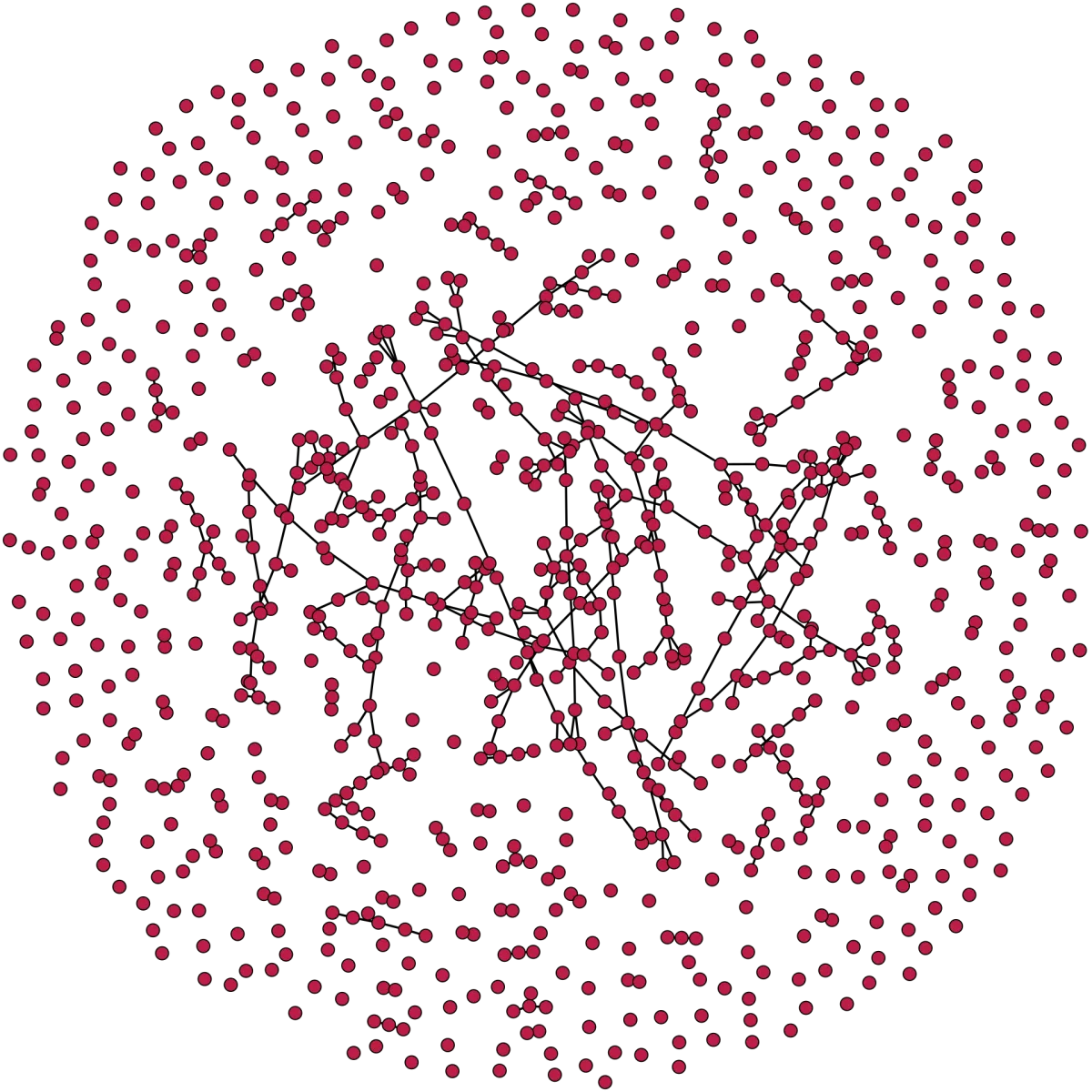
Diestel's chapter Notes add the second standard model. Instead of one coin per edge, \(G(n,M)\) deals out exactly \(M\) edges, choosing uniformly at random among all graphs on \(n\) labelled vertices with exactly \(M\) edges. This is the model Erdős and Rényi themselves worked in[6], and it behaves like \(\mathcal{G}(n,p)\) when \(M \approx p\binom{n}{2}\), the expected edge count matching up[4]. A third view makes "evolution" literal: the random graph process starts from the edgeless graph on \(n\) vertices and adds one uniformly random missing edge at a time, until the graph is complete. Its snapshot after \(M\) steps is exactly the uniform model, and the story above becomes a film you can watch frame by frame.
The threshold phenomenon itself travels far beyond graphs. Random instances of constraint-satisfaction problems, boolean satisfiability most famously, show the same behaviour: below a critical density of constraints almost all instances are solvable, above it almost none are, and the hardest instances cluster near the transition. The mathematics of Section 11.4 is the shared skeleton of all these observations.
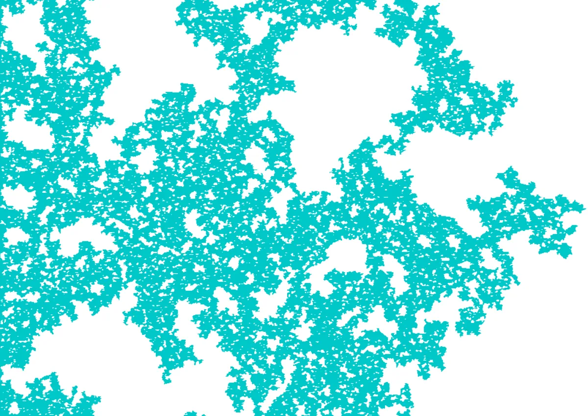
Epidemics are threshold phenomena on graphs. A disease spreading across a contact network dies out or explodes depending on whether the transmission rate crosses a critical value, and the "explodes" outcome is precisely the emergence of a giant connected component of infection, the same transition Erdős and Rényi found at \(p \approx 1/n\)[6]. Newman showed that the standard susceptible-infective-removed epidemic models can be solved exactly on a wide variety of random networks, turning outbreak questions into structural questions about the graph[8]. There is also a warning in the fine print: Pastor-Satorras and Vespignani proved that on scale-free networks, whose degree distributions have heavy tails like many real contact and computer networks, the epidemic threshold vanishes; infections can persist at arbitrarily low transmission rates, sustained by highly connected hubs, which is why hub-targeted interventions are disproportionately effective[9]. The classical model's uniform randomness is an assumption, not a law, and knowing exactly what \(\mathcal{G}(n,p)\) predicts is what makes the deviations visible.
Where to go from here: the second-moment method, threshold functions, and the evolution story are the gateway into the modern theory of random graphs, and the giant component in particular rewards a closer look; Diestel's Notes point to the standard monographs[4]. Within this course, the probabilistic method itself is the export: it proves purely deterministic theorems in Chapter 5 (list colouring) and Chapter 9 (Ramsey theory), and thinking about "typical" graphs will return when we discuss graphs as data in the AI chapters.
As \(p\) grows, in which order do these milestones occur?
Check your understanding
In this chapter, \(\mathcal{G}(n,p)\) stands for:
The symbol \(q\) in this chapter denotes:
The falling factorial \((n)_k\) equals:
Fix a particular copy \(H'\) of a graph with 5 edges on specified vertices of \(V\). In \(\mathcal{G}(n,p)\), the probability that \(H'\) is a subgraph of the random graph \(G\) is:
Let \(X \geq 0\) count occurrences of some pattern, and suppose \(E(X) \to 0\) as \(n \to \infty\). By Markov's inequality, what follows?
The threshold function for containing a triangle is \(t(n) = n^{-1}\). For which edge probability does almost every \(G \in \mathcal{G}(n,p)\) contain a triangle?
For a constant edge probability \(p \in (0,1)\), which statement is true for almost every \(G \in \mathcal{G}(n,p)\)?
To prove that almost every graph contains a copy of \(H\) above the threshold, the chapter uses Chebyshev's inequality rather than stopping at "the expected number of copies tends to infinity". Why is the expectation alone not enough?
Using the subgraph containment theorem, the threshold function for containing a path on 4 vertices (3 edges) is:
In the proof of Erdős's girth-and-chromatic-number theorem, one vertex is deleted from each short cycle. Why delete vertices rather than edges, which would also destroy the cycles?
Sources and further reading
- R. Diestel, Graph Theory, 6th ed., Springer GTM 173 (2024), §11.1.
- R. Diestel, Graph Theory, 6th ed., Springer GTM 173 (2024), §11.2.
- R. Diestel, Graph Theory, 6th ed., Springer GTM 173 (2024), §11.3.
- R. Diestel, Graph Theory, 6th ed., Springer GTM 173 (2024), §11.4 and the chapter Notes.
- R. Diestel, Graph Theory, 6th ed., Springer GTM 173 (2024), §8.3 (the Rado graph and its uniqueness, Theorem 8.3.1).
- P. Erdős, A. Rényi, "On the Evolution of Random Graphs", Publications of the Mathematical Institute of the Hungarian Academy of Sciences 5 (1960), 17–61. Full text.
- D. J. Watts, S. H. Strogatz, "Collective dynamics of 'small-world' networks", Nature 393 (1998), 440–442. nature.com/articles/30918.
- M. E. J. Newman, "Spread of epidemic disease on networks", Physical Review E 66, 016128 (2002). arXiv:cond-mat/0205009.
- R. Pastor-Satorras, A. Vespignani, "Epidemic spreading in scale-free networks", Physical Review Letters 86, 3200 (2001). arXiv:cond-mat/0010317.
- M. Campos, S. Griffiths, R. Morris, J. Sahasrabudhe, "An exponential improvement for diagonal Ramsey" (2023). arXiv:2303.09521.