Part IV · Graphs and AI
GraphRAG: Retrieval over Knowledge Graphs
Vector search answers questions whose answer lives in one passage. This chapter shows what to do when the answer is spread across an entire corpus: build a knowledge graph, find its communities with a connectivity-guaranteed algorithm, and let the graph theory you already know do the retrieval.
The question no chunk can answer
A large language model (LLM) answers from what it absorbed during training. If you want it to answer questions about your documents, the standard move is retrieval-augmented generation (RAG). The recipe has three steps. Cut the documents into chunks of a few hundred words each. Store, for every chunk, a numeric vector (an "embedding") that encodes its meaning. At question time, turn the question into a vector too, fetch the few chunks whose vectors sit closest to it, and let the model read those chunks before writing its answer.
This works well for a question like "what is the refund policy?" The answer sits in one chunk. The chunk resembles the question. Nearest-neighbour search finds it.
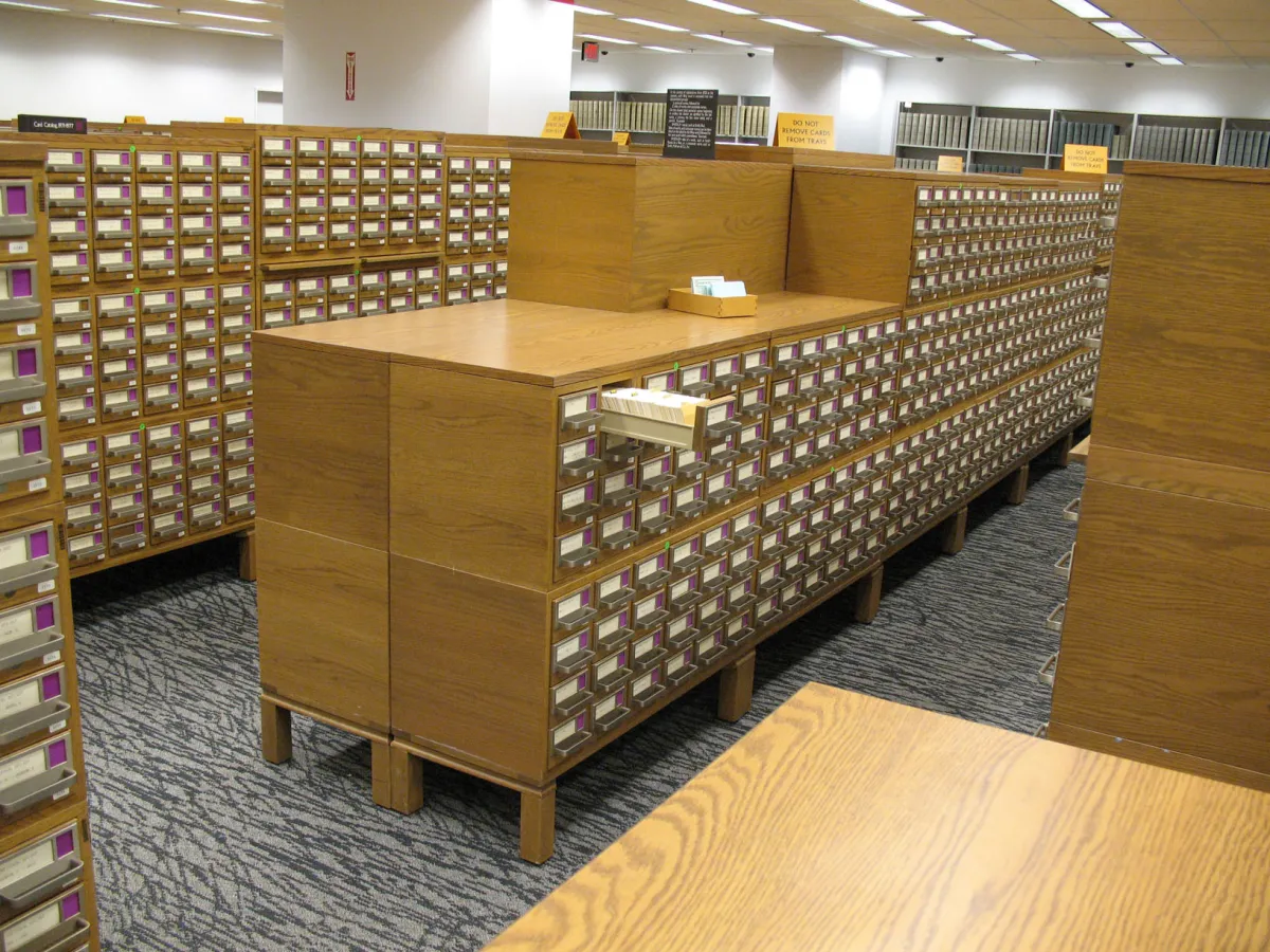
Now ask a different kind of question: "what are the main themes across this year's customer interviews?" No chunk contains the answer. The answer is a property of the whole collection, the way the average degree is a property of a whole graph and not of any single vertex. Vector similarity has nothing to grab onto, because the question does not resemble any specific piece of text. The GraphRAG paper by Edge and colleagues at Microsoft Research calls these global sensemaking questions, in contrast with local questions that a single passage can settle[1].
Microsoft's announcement post demonstrates the failure with a pair of queries over a corpus of news articles about the Russia-Ukraine war[2]. "What is Novorossiya?" is definitional and local, and both plain RAG and GraphRAG answer it. "What has Novorossiya done?" requires connecting reports scattered across many articles. Plain RAG returned nothing useful. GraphRAG answered with a list of concrete linked activities, among them plans to destroy property and to sabotage the cash machines of a named bank, each with a citation back to the source article[2].
Why did the second system succeed? Because it had edges. In the language of this course: a corpus of chunks, as vector RAG sees it, is an edgeless graph. Retrieval can rank the vertices, but there is nothing to follow. The moment you extract entities and the relations between them, "what has X done" becomes a neighbourhood query: collect the edges incident with the vertex for X and read them off. Recall the notation from Chapter 1: \(N(v)\), the neighbourhood of \(v\), is the set of vertices joined to \(v\) by an edge. The answer to the Novorossiya question is, almost literally, its neighbourhood.
GraphRAG is the family of techniques that puts a graph between the documents and the model[9]. The best-known version, from the 2024 Microsoft Research paper, runs in two stages[1]. At indexing time it extracts a knowledge graph from the text, partitions it into communities with the Leiden algorithm, and writes a summary for every community at every level of a hierarchy. At question time it answers global questions from the community summaries and local questions from vertex neighbourhoods. Every step of that pipeline is an object you have met in this course, and this chapter walks through the pipeline in that spirit: not "trust the tool," but "recognize the mathematics."
Once entities and their relationships are extracted, why does "what has Novorossiya done?" become answerable?
New notation in this chapter
Everything here builds on notation from Chapter 1 and Chapter 3, which we re-gloss as we go. Six symbols are new.
| Symbol | Read it as | Meaning | Tiny example |
|---|---|---|---|
| \(w(uv)\) | "the weight of the edge \(uv\)" | A number attached to the edge between \(u\) and \(v\), here measuring how often and how strongly two entities are linked in the text. | If two entities co-occur in 3 chunks, \(w(uv)=3\). |
| \(\mathcal{P}\) | "a partition of the vertex set" | A division of \(V(G)\) into disjoint, non-empty parts (the communities) that together cover every vertex. | \(\mathcal{P}=\{\{a,b,c\},\{d,e\}\}\) for a graph on 5 vertices. |
| \(Q(\mathcal{P})\) | "the modularity of \(\mathcal{P}\)" | A quality score for a partition: high when many edges lie inside parts and few run between them, relative to chance. | Two loose blobs joined by one edge: splitting at that edge gives high \(Q\). |
| \(G/\mathcal{P}\) | "\(G\) contracted by \(\mathcal{P}\)" | The aggregate graph: one vertex per community of \(\mathcal{P}\), with an edge between two of them when some edge of \(G\) runs between the two communities. Extends the edge contraction \(G/e\) of Chapter 1. | Contracting \(\{a,b,c\}\) and \(\{d,e\}\) gives a graph on 2 vertices. |
| \(\pi(v)\) | "the PageRank of \(v\)" | The long-run share of time a certain random walk spends at vertex \(v\); a score of how central \(v\) is. | A hub of high degree collects a large \(\pi(v)\). |
| \(\pi_S(v)\) | "the PageRank of \(v\) personalized to \(S\)" | The same walk, except the teleport step returns to the seed set \(S\); scores how reachable \(v\) is by short walks from \(S\). | With \(S=\{s\}\), the neighbours of \(s\) get large \(\pi_S\). |
Two entities are asserted to be related in three different chunks. Using this chapter's notation, how is that recorded?
From text to a knowledge graph
The indexing stage of GraphRAG turns unstructured text into a graph, and it does so with the bluntest imaginable tool: it asks the language model. Every chunk of roughly 600 tokens is sent to the LLM with a prompt that says, in effect, list the entities in this text (people, places, organizations, concepts), list the relationships between them, and describe each in a sentence[1].
A weighted graph \(G\) whose vertex set \(V(G)\) is the set of distinct entities extracted from a corpus, with an edge \(uv \in E(G)\) whenever some chunk asserts a relationship between \(u\) and \(v\), weighted by \(w(uv)\), the strength and frequency of that relationship across all chunks. In plain words: the dots are the things the documents talk about, the lines are the claims the documents make about pairs of things, and each line remembers how much text backs it up.
Two bookkeeping steps make this a graph rather than a pile of triples. First, mentions are merged: "Novorossiya", "the Novorossiya movement", and "it" (resolved from context) all become one vertex. Deciding which mentions refer to the same entity is itself a matching problem between sets of mentions, a cousin of the matchings you studied in Chapter 2, and production toolkits ship fuzzy-matching entity-resolution components for exactly this job[11]. Second, parallel edges are merged: five chunks each linking the same pair of entities become one edge of weight reflecting all five.
What do these graphs look like at real scale? The paper reports both of its test corpora[1]. A podcast-transcript corpus of about one million tokens (1,669 chunks) produced a graph with 8,564 vertices and 20,691 edges. A news corpus of about 1.7 million tokens (3,197 chunks) produced 15,754 vertices and 19,520 edges.
Recall from Chapter 1 that \(|G|\) is the order of \(G\) (its number of vertices), \(\|G\|\) is its size (its number of edges), and the average degree is \(d(G) = 2\|G\|/|G|\), because every edge contributes to the degree of exactly two vertices. For the podcast graph: \(d(G) = 2 \cdot 20{,}691 / 8{,}564 \approx 4.8\). For the news graph: \(d(G) = 2 \cdot 19{,}520 / 15{,}754 \approx 2.5\). The news graph averages barely more than two edge-ends per vertex; a tree on the same vertices would already have average degree just under 2. These graphs are only a little denser than forests.
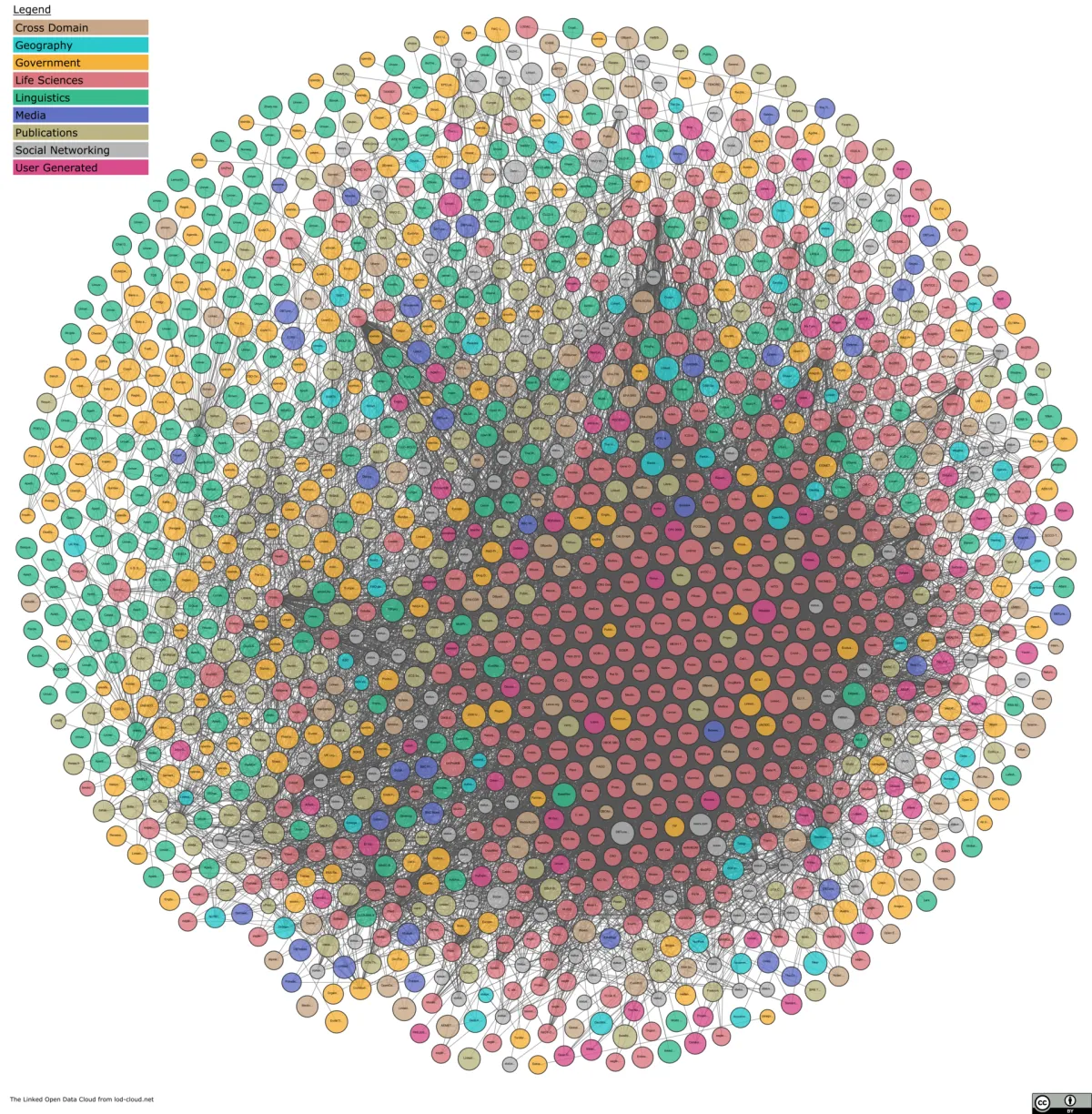
Hold on to that sparsity observation. Extracted knowledge graphs are nothing like the complete graphs of the extremal chapters. They have a few high-degree hubs (the entities the corpus keeps returning to) and a long tail of vertices of degree 1. Sparsity is what makes the next step meaningful: on a dense graph, everything is one community, and there is no structure to find.
Extracted knowledge graphs turn out to be sparse, with average degree around 2.5 to 4.8. Why does the chapter say that sparsity matters?
Communities: many edges in, few edges out
Why partition the graph at all? Because a global question needs a global summary, and you cannot summarize 8,564 entities in one pass through a context window. The plan is divide and conquer: split the graph into pieces that are internally coherent, summarize each piece, and answer from the summaries. The pieces that make this work are called communities.
A community in a graph is a set of vertices with many edges inside the set and few edges leaving it. Community detection searches for a partition \(\mathcal{P}\) of \(V(G)\) maximizing a quality score, most commonly the modularity \[ Q(\mathcal{P}) \;=\; \sum_{C \in \mathcal{P}} \left( \frac{\|G[C]\|}{\|G\|} \;-\; \left( \frac{\sum_{v \in C} d(v)}{2\|G\|} \right)^{\!2} \right), \] where \(G[C]\) is the induced subgraph on \(C\) (keep the vertices of \(C\) and every edge of \(G\) with both ends in \(C\)). Here \(d(v)\) is, as always, the degree of \(v\): the number of edges at \(v\). Read the formula aloud: for each community, take the fraction of all edges that lie inside it, subtract the fraction that a random graph with the same degrees would be expected to put inside it, and add up over communities.
Modularity asks: does this partition beat shuffling? Imagine cutting every edge in half and re-gluing the half-edges at random, so each vertex keeps its degree but loses its loyalties. A partition scores well when the real graph keeps far more edges inside the parts than the shuffled graph would. "Dense inside, sparse between" is judged against chance, not against zero.
The classic algorithm for this search is Louvain (2008). It repeats two phases. In the local-moving phase, it visits vertices and moves each one to a neighbouring community if the move improves modularity. In the aggregation phase, it contracts each community to a single vertex, so the whole graph shrinks to its quotient \(G/\mathcal{P}\), and then it runs the local-moving phase again on the smaller graph, producing coarser and coarser partitions.
Louvain has a defect that you, at this point in the course, can state precisely, and that is why we spend time on its successor. Louvain can output a "community" whose induced subgraph is disconnected. Traag, Waltman, and van Eck showed in 2019 that this is not a rare corner case: in their experiments, up to 25 percent of Louvain's communities were badly connected, and up to 16 percent were internally disconnected, with the problem worsening when the algorithm is applied iteratively[3]. Here is how it happens. A vertex \(v\) can be the only bridge between two halves of its community. Later in the run, \(v\) accumulates strong ties to a different community and moves there. The two halves it was bridging stay assigned together, but now there is no path between them inside the community. A "community" in two pieces, with no internal path from one piece to the other, is not a community in any meaningful sense.
The Leiden algorithm, named for the university where its authors work, repairs exactly this. Between the local-moving phase and the aggregation phase it inserts a refinement phase that breaks badly connected sets apart. And it comes with a proof, which is why a graph theory course gets to state it as a theorem.
Every community \(C\) output by the Leiden algorithm induces a connected subgraph: \(G[C]\) is connected. Moreover, iterating the algorithm converges to a partition in which every subset of every community is locally optimally assigned[3].
Proof idea, in the spirit of this course. The refinement phase starts from each community with every vertex in its own singleton and only ever merges a vertex into a part it is actually joined to by an edge, so each refined part grows the way a connected subgraph grows in the proofs of Chapter 1: one edge-attached vertex at a time. Since aggregation only contracts refined parts, no step ever creates a contracted vertex out of a disconnected set, and the invariant survives every iteration. The convergence claim takes more work (a potential-function argument showing each phase cannot cycle); for that, read the original paper[3]. The authors also measured it to be faster than Louvain, so the guarantee costs nothing[3].
This is the promised connection to Chapter 3, and it is not a metaphor. Connectivity, the property Chapter 3 built its whole theory on, is precisely what separates the honest algorithm from the buggy one. Two more Chapter 3 ideas are hiding here. First, the sparse edge sets between communities are small cuts: community detection is implicitly finding the small separators of the knowledge graph, the flip side of finding its dense pieces. Second, there is a contrast worth dwelling on, because it trips people up.
"A community is a highly connected subgraph." Not quite. Community quality is about edge density: many edges inside, few out, relative to chance. Chapter 3's \(k\)-connectivity (recall: \(G\) is \(k\)-connected if it has more than \(k\) vertices and stays connected after deleting any \(k-1\) of them) is about robustness to deletion. A perfectly good community can hang together by a single cut vertex, making it only 1-connected. Leiden guarantees its communities are connected; it does not, and cannot, promise any \(k\)-connectivity beyond that[3].
There is also a connection forward to Chapter 12, and it is the most satisfying one in this chapter. Both Louvain and Leiden repeatedly replace the graph by its quotient \(G/\mathcal{P}\), contracting each community to a single vertex. You know from Chapter 1 (and from Chapter 12, where the idea carried the Graph Minor Theorem) what contracting a connected vertex set means: the communities become branch sets, and the contracted graph is a minor of the original, a graph obtained by deleting vertices and edges and contracting connected pieces. Because Leiden's communities are guaranteed connected, every aggregate graph Leiden builds is a genuine minor of the knowledge graph. Under Louvain, a disconnected "community" gets contracted to one vertex anyway, and the aggregate graph carries no such guarantee, because branch sets must be connected and a disconnected community is not one[14]. The minor relation, of all things, is the exact dividing line between the two algorithms.
Modularity subtracts a term from each community's share of the edges. What is that subtracted term doing?
In Figure 14.2, Louvain leaves \(\{a,b,c,d,e,f\}\) as one community after the bridge vertex \(v\) moves into \(\{v,g,h,i\}\). What exactly is wrong with the result?
A tree of summaries
One round of Leiden gives one partition. GraphRAG runs it recursively: detect communities, then detect sub-communities inside each community, and keep going until the pieces are small enough to summarize in one model call[1]. The result is a hierarchy. The paper names its levels C0 (the root level, coarsest) down to C3 (the leaves, finest) in its experiments.
What kind of object is this hierarchy? A rooted tree, in exactly the Chapter 1 sense (a connected graph with no cycle, with one vertex distinguished as the root): its root is the whole graph, its leaves are small vertex sets, and every internal node is the union of its children. Any two communities in the hierarchy are either disjoint or nested, one inside the other; set systems with that property are called laminar, which is a stronger condition than the bags of a tree-decomposition in Chapter 12 satisfy, since those may overlap without one containing the other. The community hierarchy is the applied cousin of a tree-decomposition: a tree whose nodes cover the graph, which you descend to localize a question.
Now comes the expensive part. At indexing time, GraphRAG pays the LLM once to write a community report for every community at every level: a summary of the entities, relationships, and claims inside that community. The reports are written bottom-up, so a parent's report can be composed from its children's reports when the raw material would overflow the context window[1]. The measured sizes, for both corpora:
| Level | What it is | Podcast corpus | News corpus |
|---|---|---|---|
| C0 | Root communities, coarsest view | 34 | 55 |
| C3 | Leaf communities, finest view | 1,310 | 2,142 |
Why build the whole tree instead of just one level? Because the tree lets query time choose its resolution, and the savings are large. Answering a global question from the 34 root summaries needs 9 to 43 times fewer context tokens than map-reducing over the raw source text, and even answering from the finest level (C3) needs 26 to 33 percent fewer tokens than source-text summarization[1]. Coarse levels are cheap and broad. Fine levels are expensive and detailed. The tree is a precomputed multiscale view of the corpus, and you pick your level the way a map application picks a zoom.
Any two communities in GraphRAG's hierarchy are either disjoint or one contains the other. What structure does that property give the hierarchy?
Asking questions: global, local, and DRIFT
With the index built, GraphRAG has two query modes, plus a hybrid added later. Which mode you want depends on which graph object your question lives on.
Global search handles the corpus-shaped questions that started this chapter. Given a question, it does not touch the raw chunks at all. It takes every community report at a chosen level, shuffles them into batches, and asks the LLM, in parallel, to answer the question from each batch, scoring each partial answer's helpfulness from 0 to 100. Partial answers scoring zero are discarded; the rest are sorted by helpfulness and packed into one final context window, from which the model writes the answer. The paper calls the two stages map and reduce[1]. Notice what the graph structure already did before the query arrived: because communities have few edges between them, each report covers a nearly self-contained topic, and the map step can process reports independently without losing much. Weak coupling between parts is a cut-structure fact about the graph, put to work as parallelism.
Does it help? The paper's evaluation had LLM judges compare paired answers on four criteria: comprehensiveness (does the answer cover all aspects?), diversity (does it offer varied perspectives?), empowerment (does it help the reader judge for themselves?), and directness (is it specific and to the point, included as a control). Against vector-RAG baselines, global search won on comprehensiveness 72 to 83 percent of the time on the podcast corpus and 72 to 80 percent on the news corpus, and won on diversity 75 to 82 percent and 62 to 71 percent respectively, all statistically significant[1]. It lost on directness, which is the honest tradeoff: a corpus-wide synthesis is rarely the shortest possible reply, and for pointed factual questions the plain method's short answers win that criterion.
Local search handles the passage-shaped questions. For "what did person X say about topic Y," it embeds the question, matches it to entities in the knowledge graph, and assembles context from those seed vertices outward: their incident edges, their community reports, and the source chunks they were extracted from[4]. In course terms this is neighbourhood expansion: start from the seeds, take \(N(v)\), then vertices at distance 2 (recall \(d(u,v)\), the length of a shortest \(u\)–\(v\) path, from Chapter 1), until the context budget is spent. It is a breadth-first exploration of a ball around the seeds.
DRIFT search (Dynamic Reasoning and Inference with Flexible Traversal), added by Microsoft in October 2024, hybridizes the two modes[5]. Phase one, the primer, compares the question against the most relevant community reports and produces a draft answer plus a list of follow-up questions. Phase two runs local searches for the follow-ups, refining the draft. Phase three ranks everything into one answer. In Microsoft's tests, DRIFT beat plain local search on comprehensiveness 78 percent of the time and on diversity 81 percent[5]. Read it with Chapter 12 glasses: DRIFT starts its traversal in the contracted minor (the community level) and descends into the original graph only where the query points. That is exactly how one should navigate a graph that comes equipped with a hierarchy of contractions.
Global search shuffles the community reports into batches and answers from each batch independently, in parallel. Which fact about the communities makes that reasonable?
A user asks "what did Chen say about pricing in the March interviews?" Which mode fits, and what does it do?
HippoRAG: retrieval as a random walk
Community summaries are one way to use the graph. The other landmark 2024 system, HippoRAG, from Ohio State and Stanford, uses it in a way that will please anyone who enjoyed Chapter 11: it retrieves by running a random walk[7].
HippoRAG builds an open knowledge graph of extracted subject-relation-object triples at indexing time, with no fixed schema and no community reports. All the interesting work happens at query time. The system identifies the entities named in the question, places them as seeds, and runs Personalized PageRank from them.
Consider a random walk on \(G\): a walker at vertex \(v\) usually steps to a random neighbour (chosen through the incident edges), and occasionally teleports: it abandons the walk and restarts at a random vertex. The PageRank \(\pi(v)\) is the long-run fraction of time the walker spends at \(v\). In the personalized version, the teleport step does not restart uniformly at random but always returns to a chosen seed set \(S\); the resulting score \(\pi_S(v)\) measures how reachable \(v\) is by short walks from \(S\). In plain words: pour probability onto the seeds, let it seep along edges, keep pulling it back home, and see where it pools.
Why is this the right tool for multi-hop questions? Take "which university did the author of paper X attend?" The answer chains two facts that may live in two different documents: paper X was written by some author \(A\), and \(A\) attended some university \(U\). In the knowledge graph, that chain is a path of length 2, a two-edge walk. Vector retrieval struggles because no single chunk resembles the whole question. An iterative LLM pipeline can decompose the question and retrieve twice, but that costs a loop of model calls. HippoRAG instead lets the walk do the hopping: probability mass flows from the seed "paper X" through the author vertex, and from any university-related seed back toward the same bridge. Vertices lying on many short walks from the seeds collect high \(\pi_S\) scores, and the passages attached to the top-scoring vertices are what gets retrieved. One linear-algebra computation crosses all the hops at once.
The measured results back the design: up to 20 percent improvement over existing retrieval methods on multi-hop question answering, and answer quality comparable to or better than the iterative multi-step retrieval baseline (a method called IRCoT) while being 10 to 30 times cheaper and 6 to 13 times faster at query time, because one Personalized PageRank computation replaces a loop of LLM calls[7]. The paper frames all this in neuroscience terms (the graph plays the role of the hippocampus, an index over memories stored elsewhere), but the retrieval engine underneath is a random-walk computation, pure and simple.
Two course connections are worth making explicit. First, Chapter 11 randomized the graph and asked what properties almost surely hold; PageRank keeps the graph fixed and randomizes the walker. They are the two natural ways to put probability on a graph, and both turn hard global questions into averages. Second, \(\pi_S(v)\) is a soft, probabilistic cousin of the distance and connectivity notions of Chapters 1 and 3: a high score means many short, well-trodden routes from \(S\) to \(v\). Menger's theorem (Chapter 3: the maximum number of disjoint paths between two vertex sets equals the minimum size of a separator between them[14]) explains why this redundancy matters in practice: extraction is noisy, and a wrongly extracted or missing edge does not break retrieval when independent paths carry walk probability around the gap.
A follow-up system, HippoRAG 2, kept the Personalized PageRank engine and integrated the source passages more deeply into the graph. It targets the original's known weakness: graph-based methods used to lose to plain embeddings on simple factual questions even while winning on multi-hop ones. HippoRAG 2 reports a 7 percent improvement on associative (multi-hop) memory tasks over the strongest embedding model while matching it on factual recall[8].
What distinguishes the personalized score \(\pi_S(v)\) from ordinary PageRank \(\pi(v)\)?
Extraction missed one relationship, so an edge that should be there is absent. Why can this retrieval method still score the right vertex highly?
LazyGraphRAG: keep the graph, skip the bill
Full GraphRAG has a weak spot, and it is money. Indexing costs an LLM call per chunk for extraction, plus an LLM call per community for report writing, all before anyone has asked a single question. Microsoft's own repository warns about it in unusually blunt terms: "GraphRAG indexing can be an expensive operation, please read all of the documentation to understand the process and costs involved, and start small"[4].
LazyGraphRAG, announced in November 2024, removes almost all of that cost, and the way it does so carries a lesson about where the value in this whole architecture actually sits[6]. Its indexing stage uses no LLM at all. Lightweight text processing extracts noun phrases, and the graph is built from noun-phrase co-occurrence: two concepts are joined by an edge when they appear together. Community detection still runs on this concept graph. But no summaries are written in advance. All LLM work is deferred to query time (that is the "lazy," in the programming-language sense of computing nothing before it is demanded), where an iteratively deepening search over communities and text snippets decides, under a tunable relevance-test budget, which text is worth showing the model.
The co-occurrence construction deserves a course footnote. Noun phrases and chunks form a bipartite incidence structure (recall from Chapter 1: a bipartite graph has its vertices in two classes, with edges only between classes; here, a noun phrase is joined to every chunk containing it). The concept graph is the one-mode projection: join two noun phrases when they share a chunk neighbour. Many useful graphs are derived graphs in exactly this way.
The measured claims, on a corpus of 5,590 Associated Press news articles with 100 synthetic queries[6]: indexing cost is comparable to plain vector RAG and about 0.1 percent of full GraphRAG's; at query cost comparable to vector RAG, LazyGraphRAG beats all competing methods on local queries; it matches GraphRAG global search's answer quality at more than 700 times lower query cost; and at 4 percent of the global-search query cost it significantly outperforms all comparison conditions on both local and global queries.
The lesson for a graph theory student: the value was never in the LLM-written labels. It was in the graph structure, which cheap statistics recover well enough for community detection to do its job. The expensive model is best spent at query time, on the few pieces of text the structure has already singled out.
LazyGraphRAG joins two noun phrases whenever some chunk contains both. In Chapter 1 terms, the resulting concept graph is:
What it costs, what you get, and what runs in production
By 2025-2026 the head-to-head evaluations had caught up with the excitement, and the honest summary is that graph-based RAG is a tool with a domain of application, not a strict upgrade. The most useful single source is the systematic comparison by Han and colleagues, which standardized preprocessing, retrieval, and generation across methods before measuring[10]. Their findings sort cleanly along a graph-theoretic axis: ask which object of the graph your question lives on.
| Question shape | Graph object | Who wins |
|---|---|---|
| Single-hop factual lookup | A vertex (one chunk) | Plain vector RAG[10] |
| Multi-hop chain | A path | Graph methods: HippoRAG 2, GraphRAG local search[10] |
| Corpus-wide themes | The partition structure | Community-based global search for coverage; plain RAG for matching reference summaries word-for-word[10] |
The costs are just as clean. On the MultiHop-RAG benchmark, building the community-based GraphRAG index took 5,560 seconds against 135 seconds for plain RAG: a 41-fold gap, and some knowledge-graph variants also paid heavy retrieval latency[10]. Put that next to the quality numbers from the original paper (comprehensiveness win rates of 72 to 83 percent on global questions[1]) and the cost numbers from LazyGraphRAG (about 0.1 percent of the indexing cost while matching global-search quality[6]), and the design space collapses to one sentence: pay for structure when your questions need structure, and when the indexing budget is the constraint, derive the graph cheaply and defer the model to query time.
GraphRAG left the lab quickly. Microsoft's reference implementation is open source under the MIT license at github.com/microsoft/graphrag, with about 35,600 stars as of August 2026; it ships the full pipeline (extraction, Leiden communities, report generation, and local, global, and DRIFT search) and is now in maintenance mode, with new research energy going to successors like LazyGraphRAG[4]. Neo4j, the main graph-database vendor, ships a first-party Python package with knowledge-graph construction pipelines and a menu of retrievers[11]. LlamaIndex ships a property-graph index whose retrieval composes vector search over graph nodes with path traversal from selected vertices[12]. LangChain's Neo4j integration provides a text-to-graph transformer and a chain for natural-language querying of the graph[13].
One item from that toolbox earns a final course connection. Neo4j's Text2Cypher retriever translates a natural-language question into a query in Cypher, the graph-database query language, whose patterns look like (a)-[:WORKS_FOR]->(b)[11]. Executing such a query means finding all the places where a small pattern graph embeds into the big host graph. That is subgraph pattern matching: a computational cousin of the subgraph containment questions running through this course, and for hard patterns it is NP-hard (no known algorithm handles every case efficiently), for exactly the reason finding large cliques is hard. Even the query language, in the end, is asking one of our questions.
So here is the chapter in one paragraph. Vector retrieval fails on global questions because a corpus without edges is an edgeless graph. GraphRAG adds the edges (an LLM-extracted, weighted, sparse knowledge graph), finds its dense pieces with an algorithm whose headline guarantee is a connectivity theorem, organizes the pieces into a rooted tree of summaries whose nesting is laminar, and answers global questions from the tree and local questions from neighbourhood balls. HippoRAG replaces summaries with a personalized random walk whose scores are soft connectivity. LazyGraphRAG shows the structure mattered more than the labels. Chapters 1, 2, 3, 11, and 12 of a pure mathematics book turn out to be the parts list of a 2024-2026 retrieval stack.
Running a Cypher pattern such as (a)-[:WORKS_FOR]->(b) against a graph database amounts to which problem?
Check your understanding
How do you read the symbol \(\pi_S(v)\), as used in this chapter?
A user asks "what are the main themes across these 3,000 customer interviews?" Why does plain vector RAG perform poorly on this question?
The podcast knowledge graph in the GraphRAG paper has \(|G| = 8{,}564\) vertices and \(\|G\| = 20{,}691\) edges. Using \(d(G) = 2\|G\|/|G|\), its average degree is about:
GraphRAG uses the Leiden algorithm instead of Louvain for community detection. What specific guarantee motivated Leiden's design?
Leiden's aggregation phase contracts each community to one vertex, giving \(G/\mathcal{P}\). Why is this aggregate graph a minor of the knowledge graph?
How do you read \(G/\mathcal{P}\)?
In the GraphRAG paper's experiments, answering global questions from root-level (C0) community summaries instead of map-reducing over the raw source text changed context-token usage how?
"Which university did the author of paper X attend?" spans two documents. How does HippoRAG retrieve for it in a single step?
LazyGraphRAG cuts indexing cost to about 0.1 percent of full GraphRAG's. What does it change?
According to the standardized head-to-head evaluation of RAG against GraphRAG methods, where does plain vector RAG still win?
Sources and further reading
- D. Edge, H. Trinh, N. Cheng, J. Bradley, A. Chao, A. Mody, S. Truitt, D. Metropolitansky, R. O. Ness, J. Larson, "From Local to Global: A Graph RAG Approach to Query-Focused Summarization" (2024). arXiv:2404.16130.
- J. Larson, S. Truitt, "GraphRAG: Unlocking LLM discovery on narrative private data," Microsoft Research blog, February 13, 2024. microsoft.com/research.
- V. A. Traag, L. Waltman, N. J. van Eck, "From Louvain to Leiden: guaranteeing well-connected communities," Scientific Reports 9:5233 (2019). arXiv:1810.08473.
- Microsoft, microsoft/graphrag (open-source GraphRAG pipeline, MIT license). github.com/microsoft/graphrag.
- J. Whiting, Z. Hills, A. Guevara Fernández, H. Trinh, A. Bradley, J. Larson, "Introducing DRIFT Search: Combining global and local search methods to improve quality and efficiency," Microsoft Research blog, October 31, 2024. microsoft.com/research.
- D. Edge, H. Trinh, J. Larson, "LazyGraphRAG: Setting a new standard for quality and cost," Microsoft Research blog, November 25, 2024. microsoft.com/research.
- B. Jiménez Gutiérrez, Y. Shu, Y. Gu, M. Yasunaga, Y. Su, "HippoRAG: Neurobiologically Inspired Long-Term Memory for Large Language Models," NeurIPS 2024. arXiv:2405.14831.
- B. Jiménez Gutiérrez, Y. Shu, W. Qi, S. Zhou, Y. Su, "From RAG to Memory: Non-Parametric Continual Learning for Large Language Models" (HippoRAG 2), ICML 2025. arXiv:2502.14802.
- B. Peng, Y. Zhu, Y. Liu, X. Bo, H. Shi, C. Hong, Y. Zhang, S. Tang, "Graph Retrieval-Augmented Generation: A Survey" (2024). arXiv:2408.08921.
- H. Han, L. Ma, Y. Wang, H. Shomer, Y. Lei, Z. Qi, K. Guo, Z. Hua, B. Long, H. Liu, C. C. Aggarwal, J. Tang, "RAG vs. GraphRAG: A Systematic Evaluation and Key Insights" (2025-2026). arXiv:2502.11371.
- Neo4j, neo4j-graphrag-python (first-party Neo4j GraphRAG package, Apache 2.0: knowledge-graph construction, entity resolution, vector, hybrid, and Text2Cypher retrievers). github.com/neo4j/neo4j-graphrag-python.
- LlamaIndex, "Property Graph Index," LlamaIndex documentation. developers.llamaindex.ai.
- LangChain, langchain-neo4j (v0.10.0, June 2026: LLMGraphTransformer, Neo4jVector, GraphCypherQAChain). pypi.org/project/langchain-neo4j.
- R. Diestel, Graph Theory, 6th ed., Springer GTM 173 (2024), §1.5 (trees), §1.7 (contraction and minors), §3.3 (Menger's theorem), Ch. 11 (random graphs), Ch. 12 (minors and tree-decompositions).